Microscopy Basic Training
This is the textbook for the microscopy basic training course that is provided to new members of the Laboratory of Experimental Biophysics at the École Polytechnique Fédérale de Lausanne (EPFL), Switzerland.
The course grew out of a yearly survey of lab members asking about problems and inefficiencies in their research. Participants indicated that they felt underprepared to address unexpected technical problems that arise during imaging experiments. These problems are further compounded by the fact that the lab uses a mixture of custom and commercial microscopes and software. In addition, we are a multidisciplinary lab with a range of backgrounds and experience, so our communal knowledge tends to be dispersed among our members. As a result it is often difficult to find the right person to help.
The EPFL BioImaging and Optics Platform (BIOP) provides a yearly course in advanced microscopy. At the time of this basic training’s conception, those students who had attended the BIOP course felt that it was useful, but too focused on theoretical aspects of microscopy to address the problems identified in the survey. We therefore collectively decided to create our own basic training course that would complement the material covered by the BIOP, focusing on hands-on learning and problem solving.
Focus Areas
In a follow-up discussion we decided upon a list of areas that the course should emphasize:
- Microscope customization to better fit the needs of an experiment
- How to adjust microscope settings for optimal imaging
- Relationships between microscope parameters and tradeoffs
- Micro-Manager
- How to identify points of failure (software, sample, camera, etc.)
- How to describe imaging problems clearly and demonstrate a train of thought
- Asking for help effectively
Many of these skills cannot be directly taught. We hope that the problem solving scenarios that one naturally encounters when building and operating a custom-built microscope will instead serve as a sufficient environment for learning practical skills.
Structure and Duration
The course is intended to last at most two weeks with students spending a few hours per day on the material. It is divided into modules so that
- a set of modules may be chosen according to each student’s background and needs
- a module can be studied independently and as needed throughout the course of a student’s or post-doc’s time in the lab
An experienced member of the lab will provide help and feedback during the course, though free time for play is encouraged.
Corrections and Suggestions
Any corrections or suggestions may be made by opening a pull request or issue at this book’s GitHub repository: https://github.com/LEB-EPFL/basic_training
Learning Outcomes
Fluorescence (Core) Module
The core module focuses on aspects of fluorescence microscopy because it is the central tool of our lab.
At the end of this training, a student should be able to:
Identify the components of an epifluorescence microscope
- The students should know the names of the components when pointed to on the training microscope
- The students should be able to identify (approximately for hidden components) where on a real microscope the same components are located
- The students should be able to state the purpose of each component
- The students should be able to sketch a basic epifluorescence microscope from memory
Assess the relative brightnesses of fluorescence signals
- The students should be able to acquire flourescence images at high SNR without saturation by tuning the microscope parameters while at the scope
- The students should know how to remove the effects of camera offset
- The students should know how to perform background subtraction and identify when it is necessary to do so
- The students should be able to estimate how much brighter the signal is in one fluorescence channel vs. another
Optics Module
The purpose of the alignment module is to provide hands-on experience to students and post-docs who will build laboratory setups for fluorescence microscopy.
At the end of the alignment module, a student should be able to:
Build and Align Optical Systems
- The students should be able to practice basic laser safety
- The students should be able to assemble Thorlabs components into a working optical system
- The students should be able to place a camera in the focal plane of a lens
- The students should be able to align lenses to a reference axis in 3D using a laser beam
Control Microscope Hardware
- The students should be able to install and configure Micro-Manager
- The students should be able to send and receive serial commands from hardware
Live Cell Fluorescence Imaging of Mitochondria
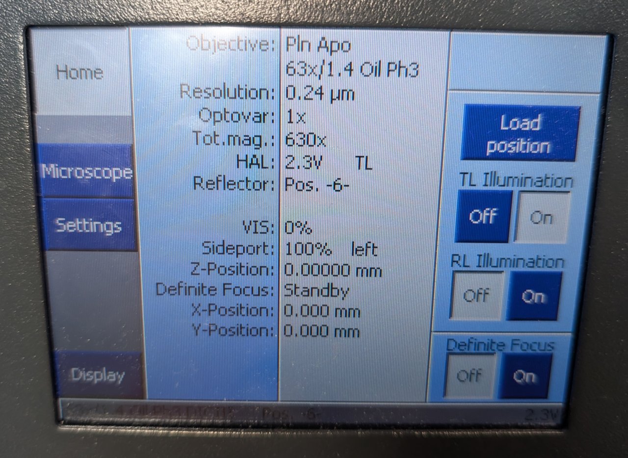
In this section we will use a Zeiss Axio Observer 7 widefield fluorescence microscope to perform live cell imaging of mitochondria in U2OS cells. The cells have been modified to express StayGold fluorescent protein that is targeting the mitochondrial matrix.
The Epifluorescence Microscope
Microscopes come in many different shapes, sizes, and arrangements. Broadly speaking, we may classify a microscope according to two different characteristics:
- The contrast mechanism
- The probe
Contrast refers to the variations of intensity within an image. Higher contrast means a greater degree of these variations, which is almost always desirable for seeing small features. We can refine this definition and go into much greater detail about what contrast means for different types of microscopes, but this would distract from our main purpose at this point, which is learning about practical microscopy.
Contrast mechanism is the physical process by which variations in intensity are generated in a microscope image. It can be either intrinsic, such as the absorption and scattering of light or other types of radiation from the sample itself, or extrinsic, such as fluorescent labels that we attach to our samples.
In nearly all forms of microscopy we need to probe our samples in order to see them. In atomic force microscopy, for example, we bring a sharp tip close to a sample’s surface to measure its height profile. In this case the probe is a very real and tangible thing. Most forms of microscopy, however, use directed beams of radiation such as light or electrons as the probe. The interaction between the radiation and the sample is ultimately what creates contrast in the image.
Light microscopy in particular refers to all forms of microscopy that use visible and near infrared light as the probe. It is probably the form of microscopy that is most used by cell biologists because light is relatively easy to manipulate and can generate very detailed images of cells with good contrast. It is also comparatively gentle on samples, enabling live cell time lapse imaging for long periods of time.
Typically there are two ways to deliver light to the sample. One is to stick the sample directly between a light source and the microscope to record the light signal that is transmitted through the sample. This geometry is called transillumination and is almost always used to probe a sample’s intrinsic contrast. The other is to illuminate and collect light from the sample through the same optical elements. This is called epi-illumination, and nearly all flourescence microscopes use it because it is much easier to separate the probe light from the fluorscence signal than it is in transillumination.
In this course you will construct and operate what is known as an epifluorescence microscope, i.e. a light microscope that illuminates the sample by epi-illumination and uses fluorescence as the extrinsic contrast mechanism.
Principle Components of an Epifluorescence Microscope
The diagram below illustrates the layout of a typical epifluorescence microscope.

You can see right away that there are two distinct, partially overlapping light paths, and the components of this microscope are positioned relative to these two paths.
The Illumination Light Path
The illumination path delivers excitation light to the sample. It is called excitation light because this light excites the flourophores to a higher energetic state, often called an excited state. The fluorophores will in turn emit fluorescence light when they relax from the excited state to the ground state.
The illumination path starts at the light source, which can be a LED, a laser, a lamp, or any other bright source of visible light. A series of optics directs this light through an excitation filter. The excitation filter absorbs light with wavelengths that are outside of the filter’s passband and transmits light with wavelengths that are inside the passband. The purpose of the excitation filter is to narrow the spectrum of the light that eventually reaches the sample. By narrowing the spectrum, we
- reduce any unwanted background signal that might leak towards the camera, and
- can better control which fluorophores are excited in the case of multi-color imaging.
Next, the light is redirected by a dichroic mirror that reflects light of some wavelengths and transmits others. The excitation light then passes through the objective lens where it is focused onto the sample to the excite fluorescence.
The Fluorescence Light Path
Fluorescence light is collected from the sample by the objective where it traverses the illumination light path in reverse. Fluorescence light has a longer wavelength than the excitation light, so it passes through the dichroic mirror instead of reflecting. An emission filter further helps remove any residual excitation light that might be traveling along this path. A normal mirror redirects the light into a different direction, though this is not necessary and is used only to reduce the overall size of the microscope.
Finally, a tube lens collects the fluorescent light and forms the image of the sample on the camera.
Microscope Startup
We will begin by starting up the microscope and its components.
Instructions
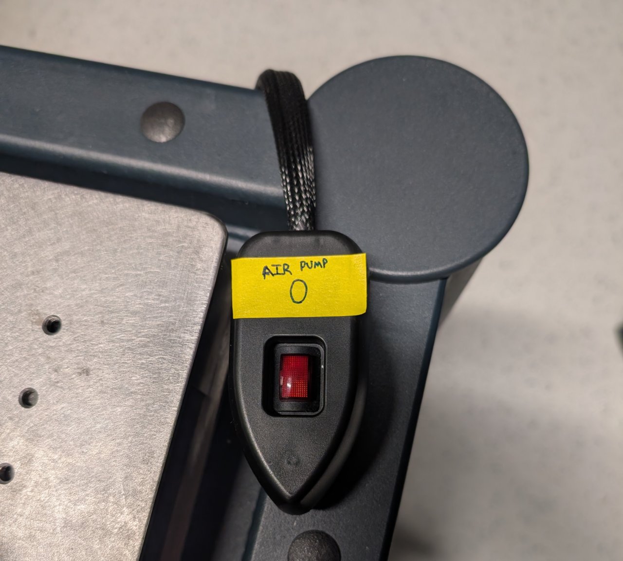
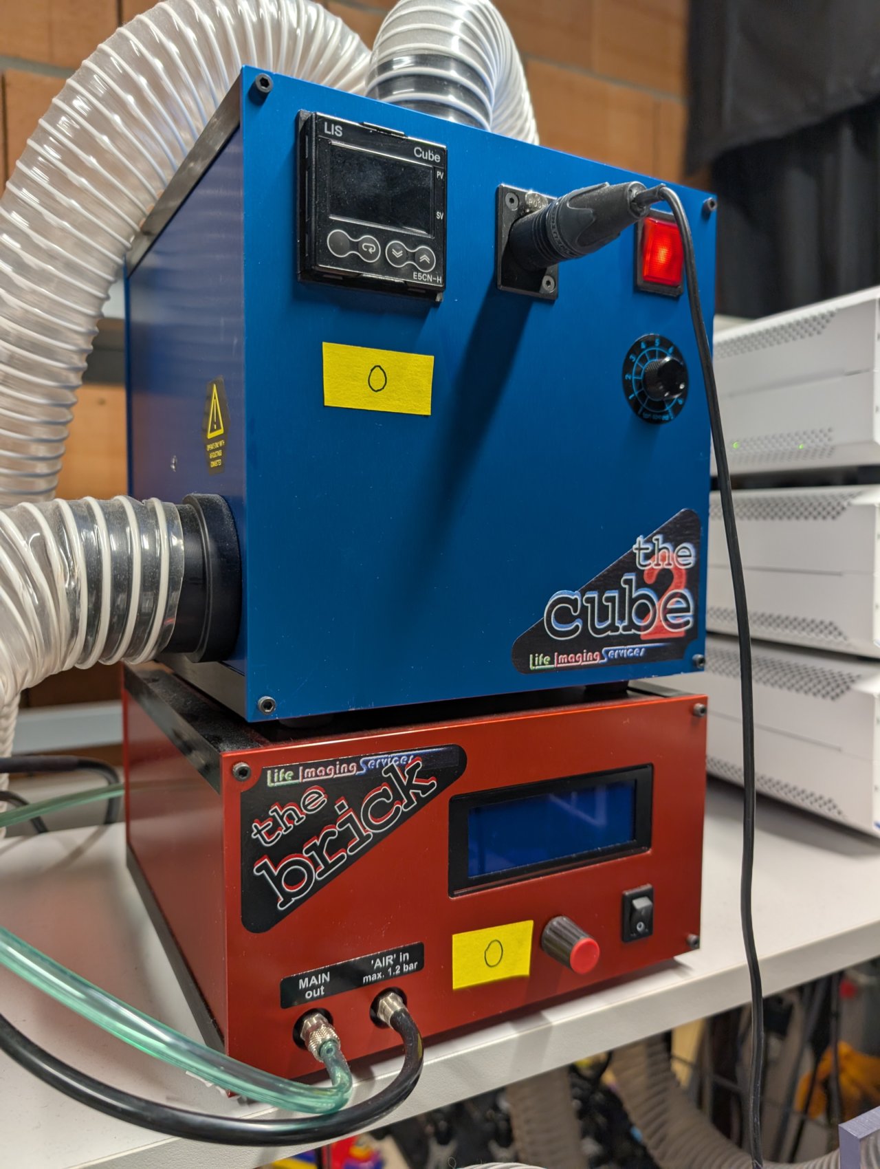
Step 0
Turn on the air pump and the environmental controls for the incubator.
It is good practice to turn these on 10 minutes or more before any experiment so that the environmental controls have a chance to stabilize.
Step 1
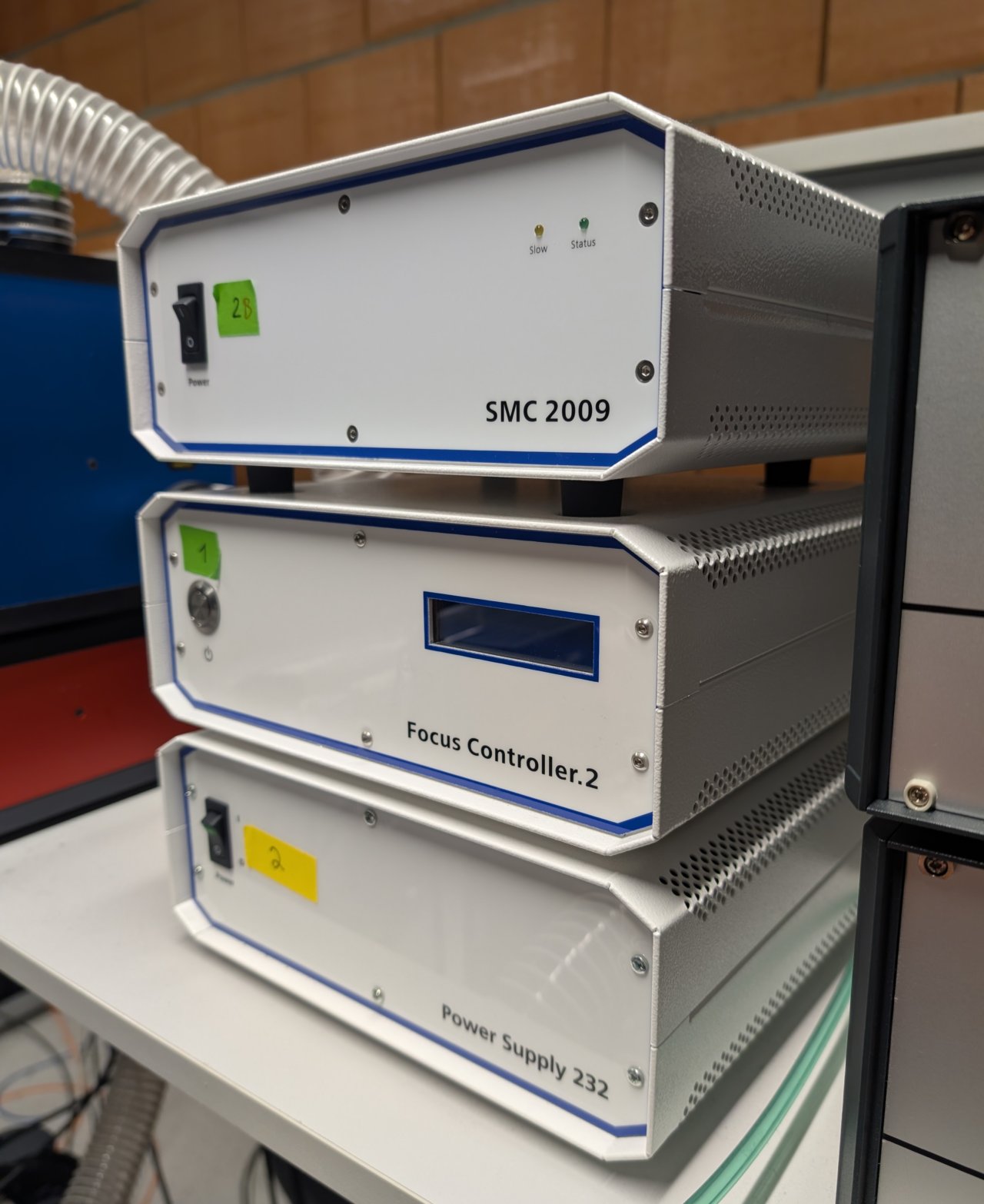
Turn on the focus controller for the Zeiss’s Definite Focus system.
In addition, turn on the Zeiss’s Power Supply 232 and SMC 2009 controllers.
Step 2
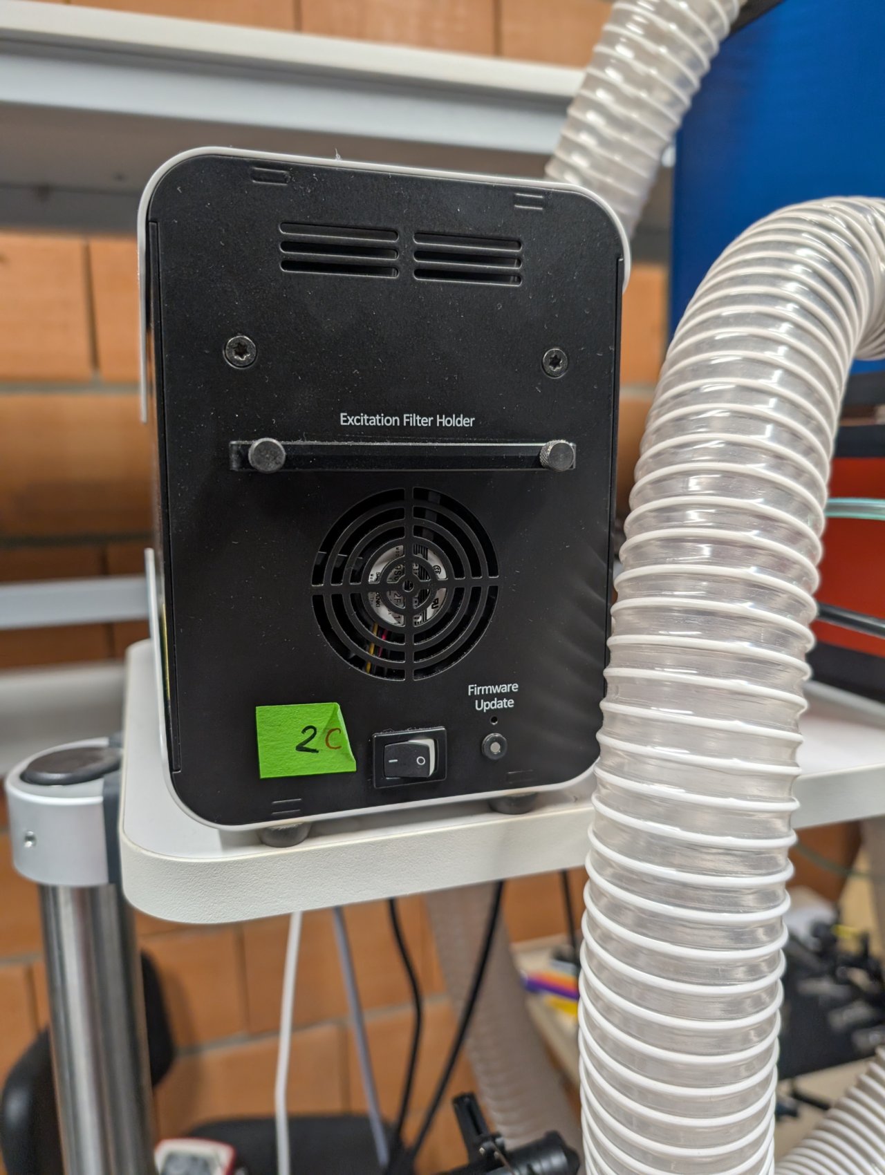
Turn on the CoolLED unit.
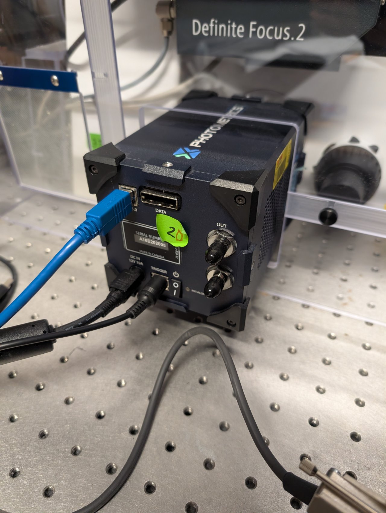
Step 3
Turn on the camera. You need not wait for the initialization to finish before turning on the control PC because the camera is connected via USB.
Step 4
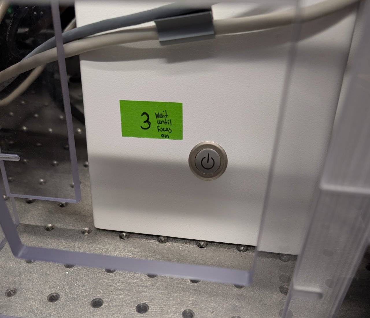
Wait until the Definite Focus controller’s initialization has finished. (You can tell whether it has finished because it will no longer display a message indicating that it is initializing on its LCD display screen.)
Turn on the microscope.
Step 5
Log into the computer with your EPFL username.
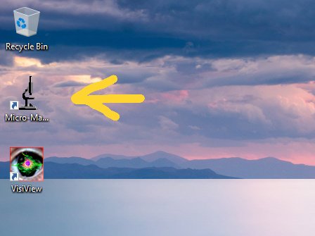
Find the shortcut to Micro-Manager on the desktop and double click it.
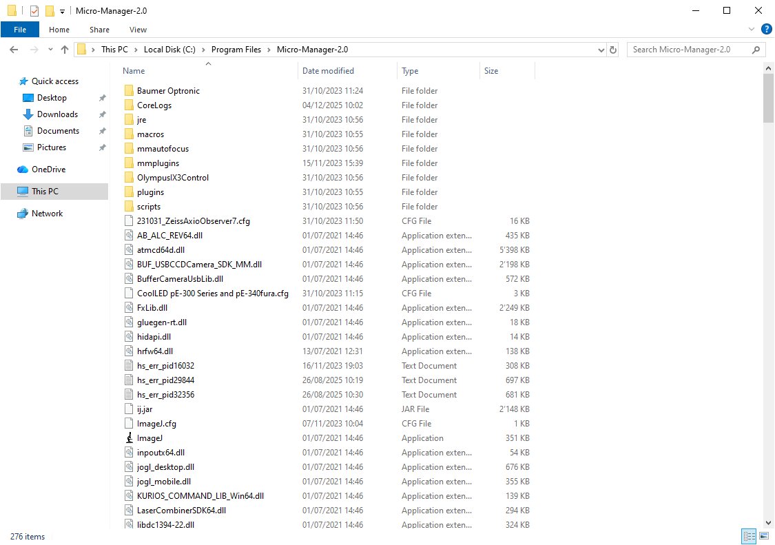
2025-12-05: This shortcut should point to C:\Program Files\Micro-Manager-2.0\ImageJ.exe. It is a slightly out-of-date version of Micro-Manager that is intended to support the CoolLED light source.
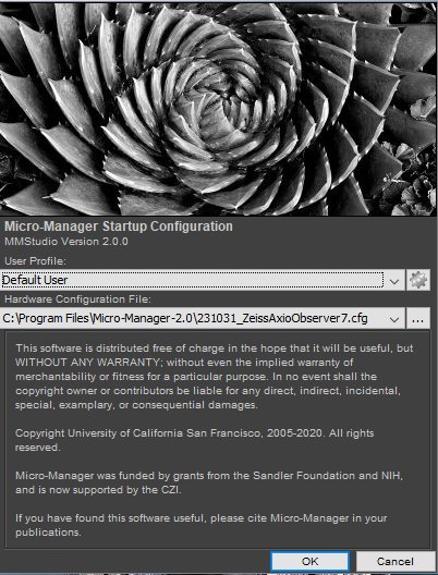
Step 6
After a few seconds or less You will see the Micro-Manager startup screen. Ensure that the 231031_ZeissAxioObserver7.cfg configuration file is selected. We have placed it inside the Micro-Manager folder in case you must select it yourself.
Click OK to continue.
Step 7
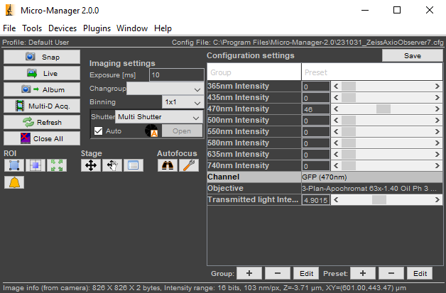
After a few more seconds, you will see the Micro-Manager control panel. If you do not see all the configuration settings at first, then expand the window by dragging its border.
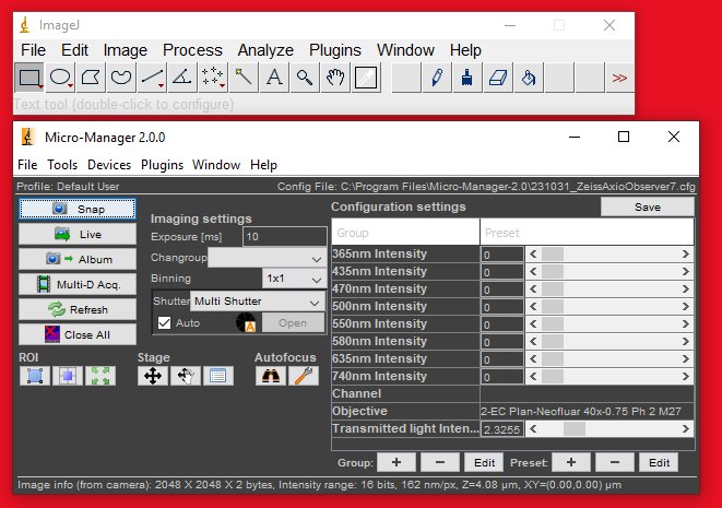
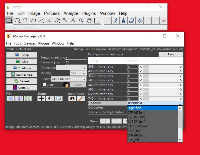
Step 8
You can set the channel and objective by selecting the corresponding configuration settings in the control panel.
Step 9
Click the Live button. If you see a noisy image stream appear, then you are ready to proceed to the next steps.
Step 10
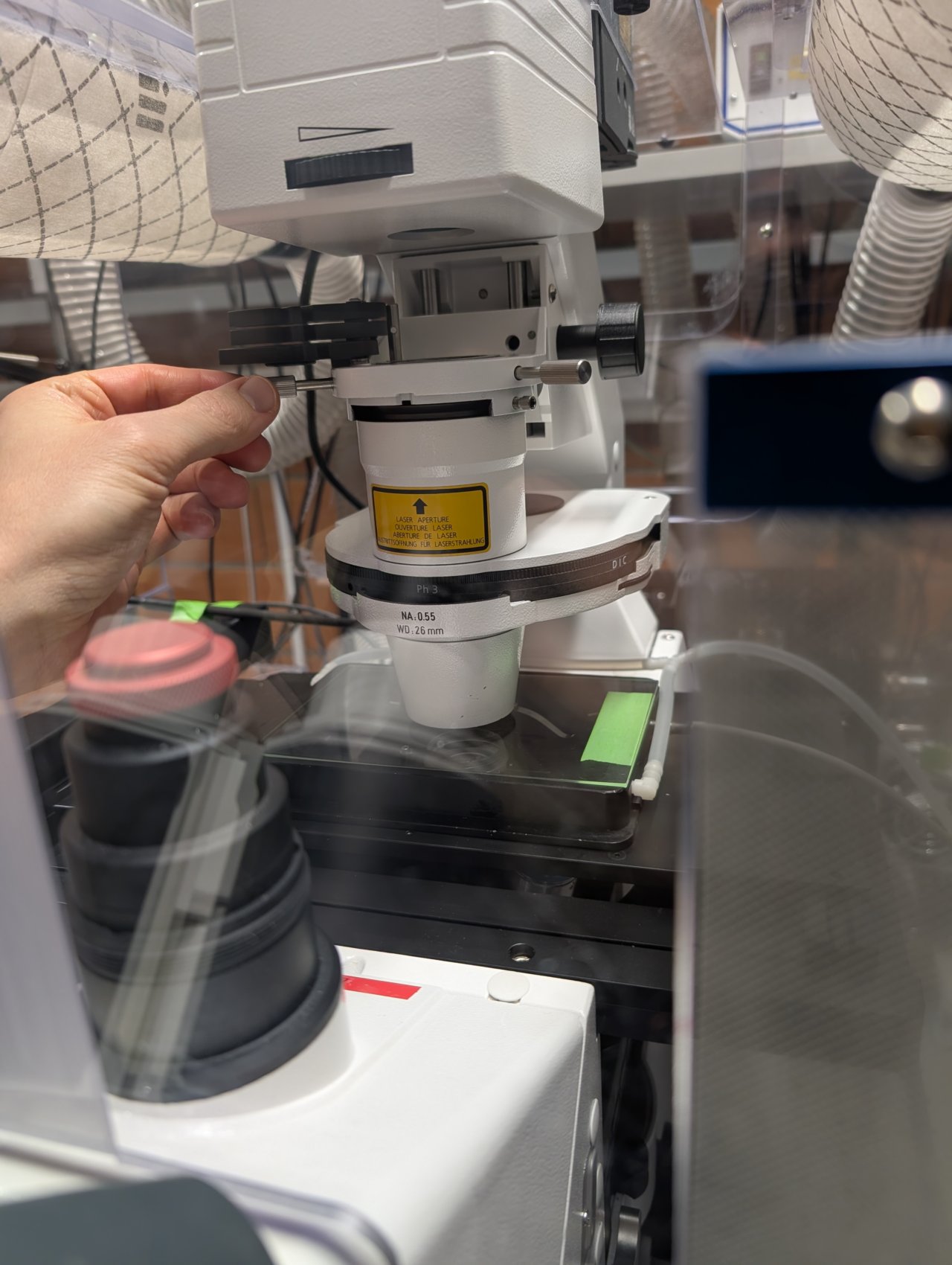
Push back the condenser tower. It is a bit difficult and does not rotate easily.
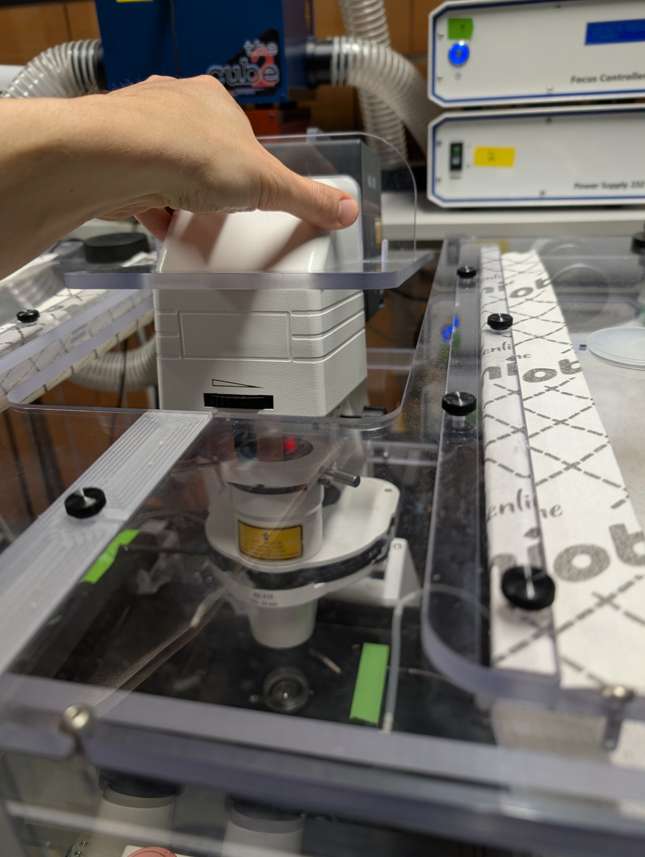
Step 11
Make sure that you are using the 63x oil immersion objective. If not, use the control panel to switch to it.
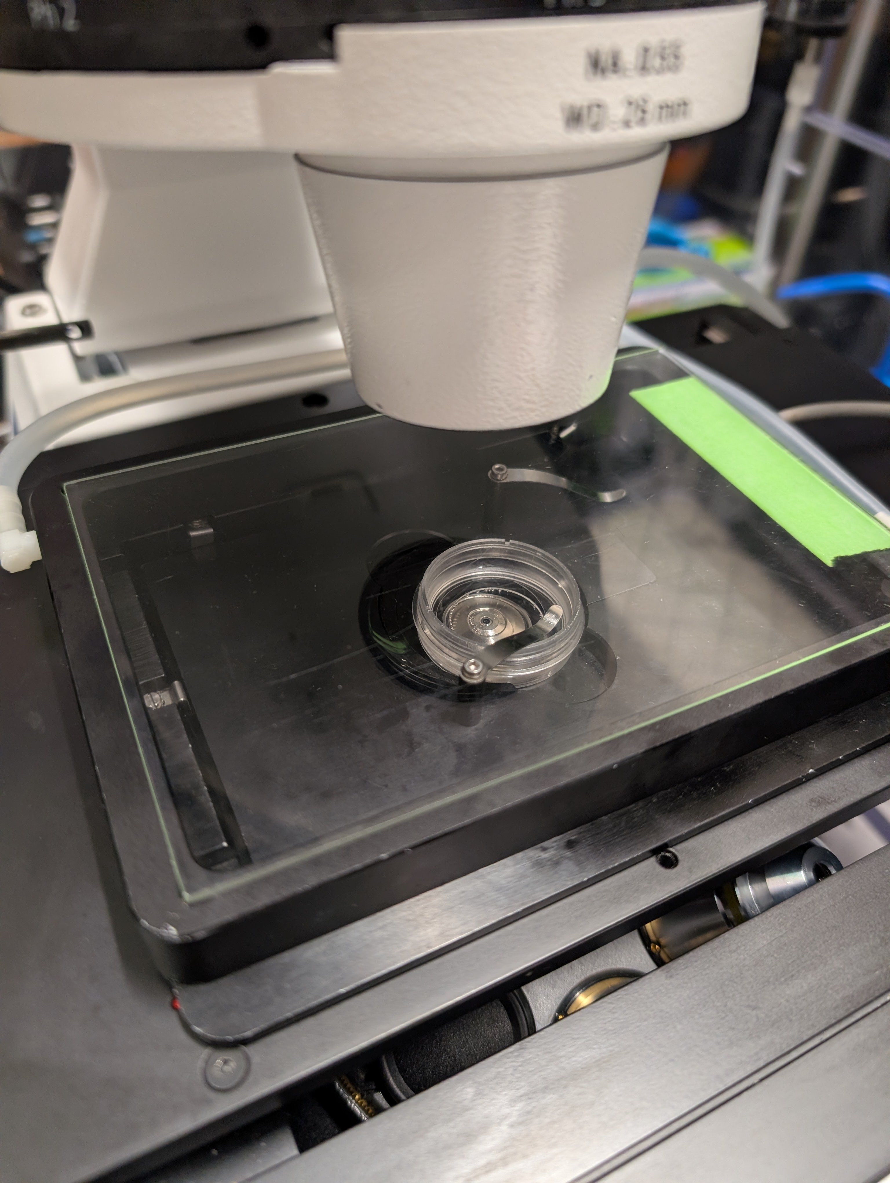
Add a small drop of 37 C immersion oil to the lens, and put your sample in the solid bottom plate. Put the plate into the opening in the microscope stage.
Secure the sample dish with a metal clip.
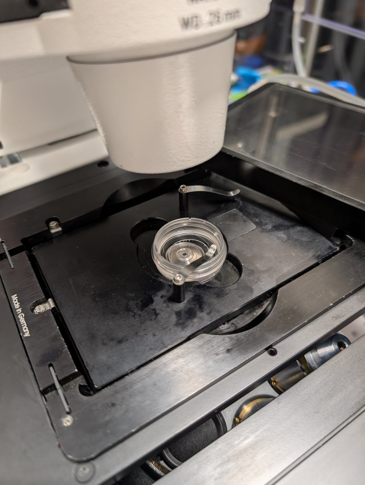
Step 12
Cover the sample dish with the CO2 chamber.
Set up Köhler Illumination
This section assumes that the microscope is on and your sample is on the stage.
We will align the condenser tower so that the sample is illuminated with Köhler illumination. Köhler illumination refers to a specific configuration of the transillumination optics that ensures:
- homogeneous illumination
- field-independent image quality
In addition, we will ensure good alignment for phase contrast imaging.
Instructions
Step 0
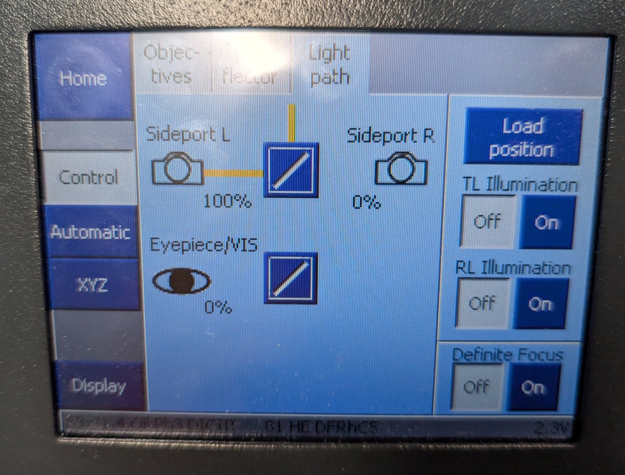
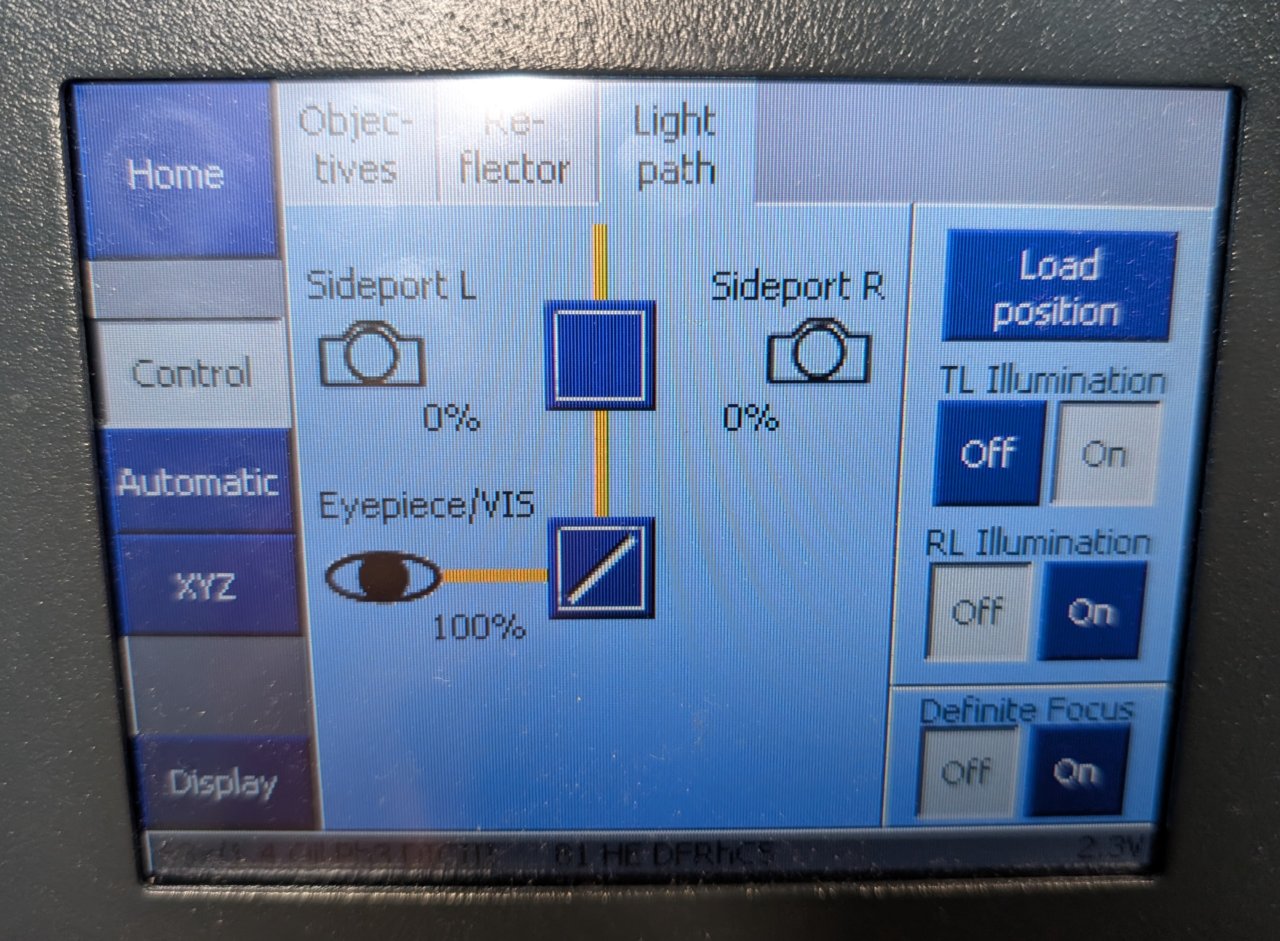
Under the Light Path tab of the Zeiss control panel, switch the light path from sideport to eyepiece.
Step 1
Open the field stop of the condenser until it is full open.
Step 2
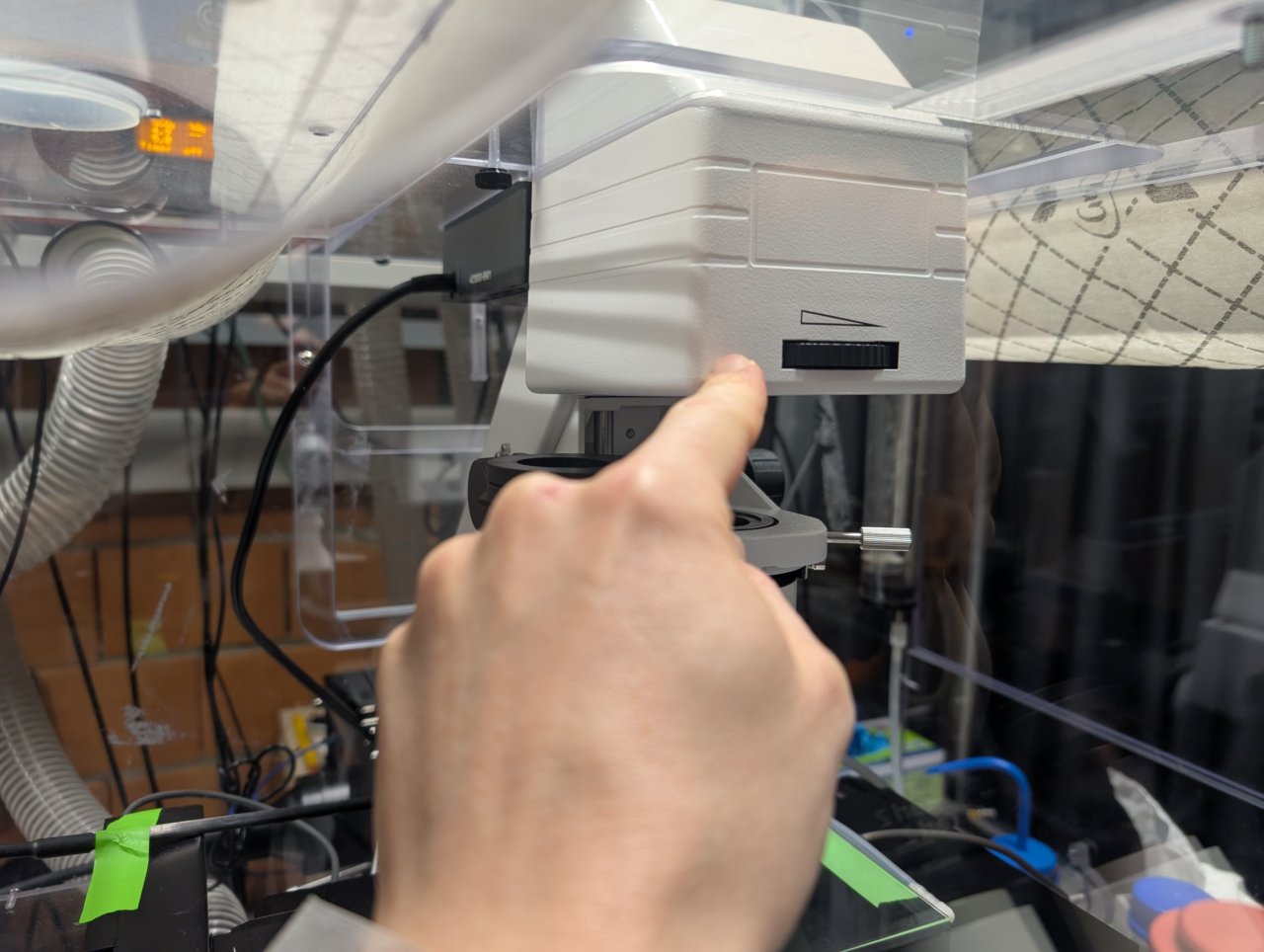
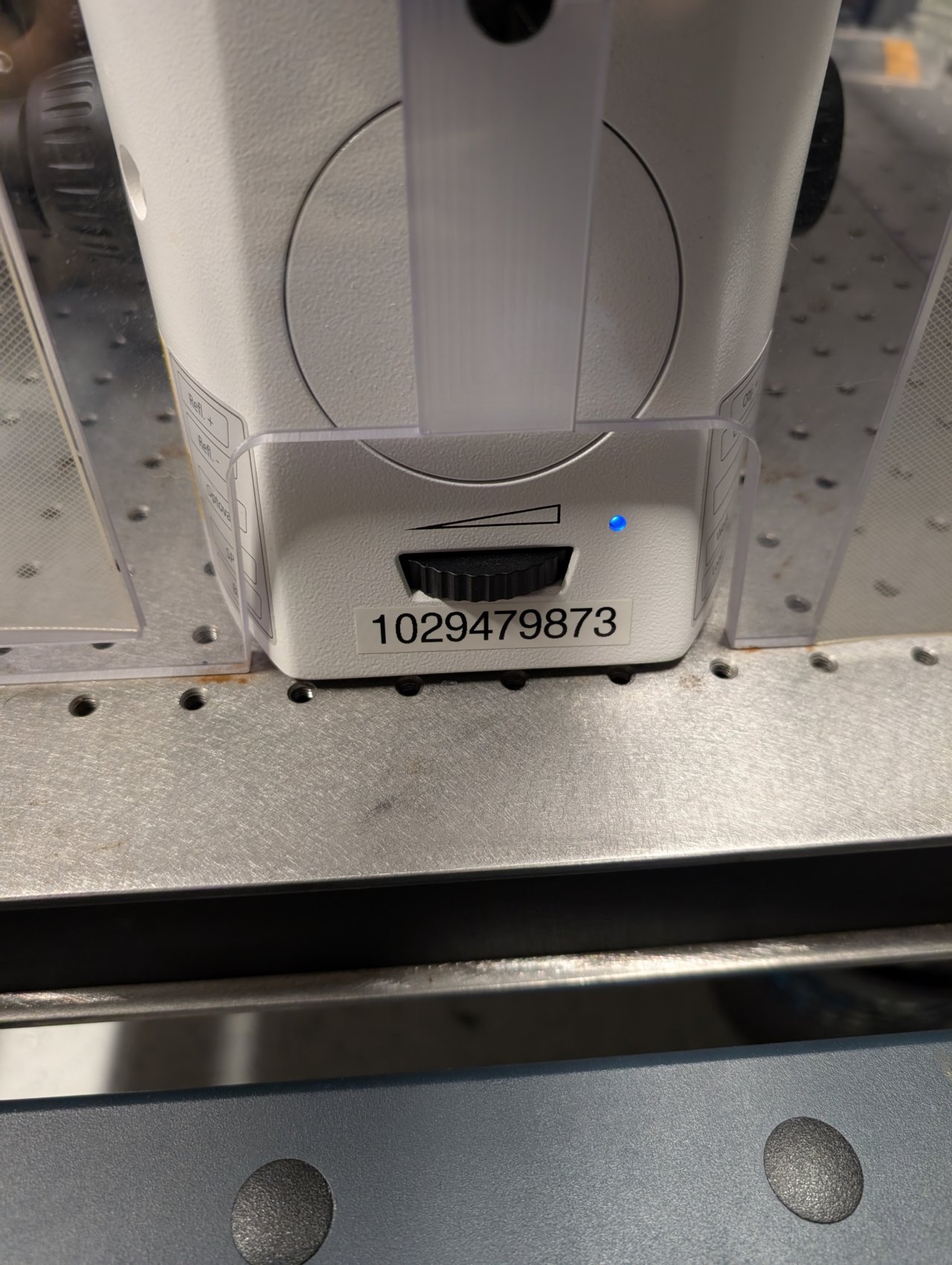
Adjust the illumination intensity. Turn the focus knobs on the microscope until the sample is brought into focus.
Do not proceed to the next step until you are focused on the sample.
Tip: Depending on their confluency, you may need to translate the stage to find an area containing cells.
If you are having trouble focusing, trying translating the sample and looking for changes in the field of view first. You can tell if cells are there even if they are out-of-focus.
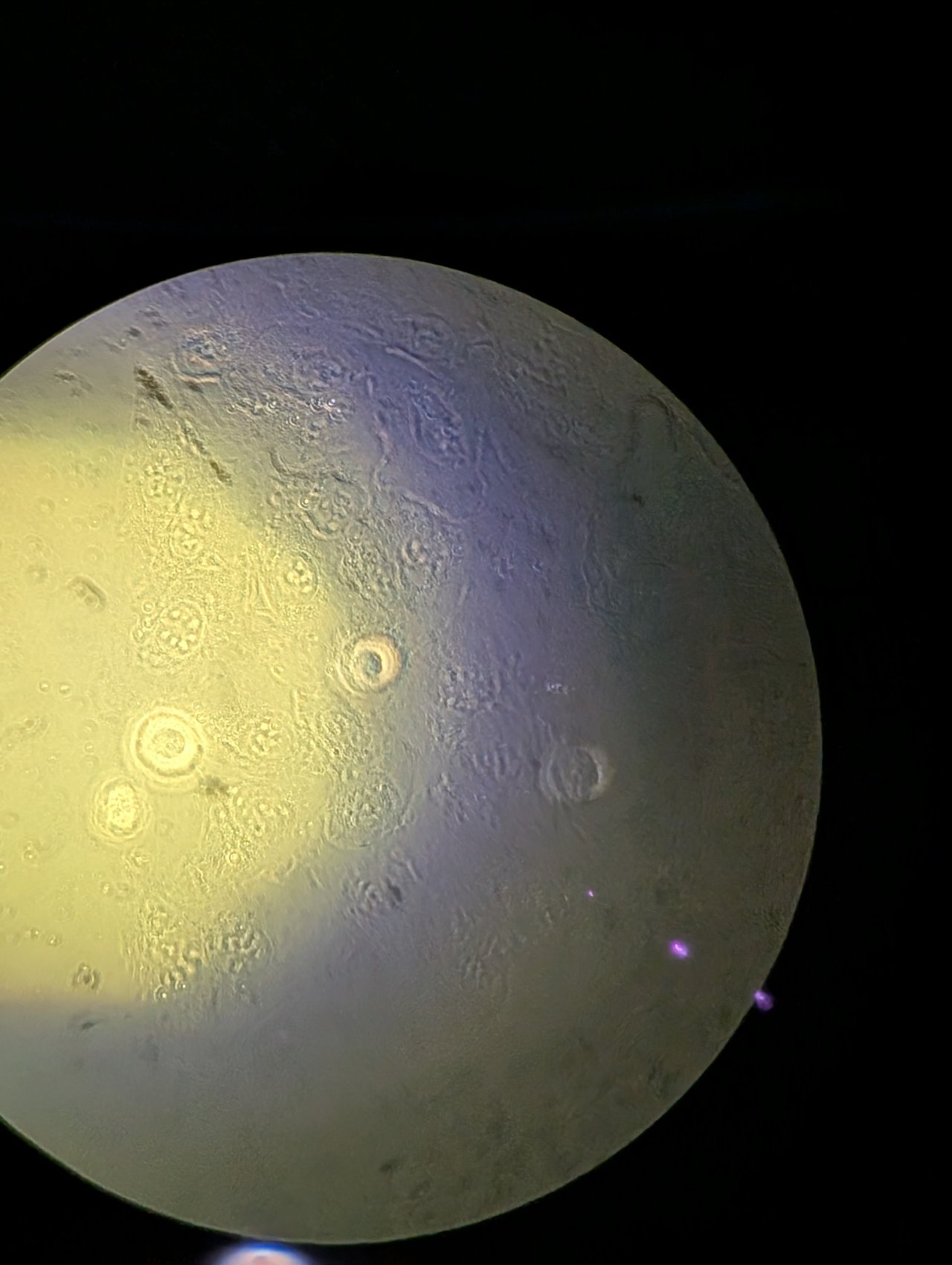
Step 3
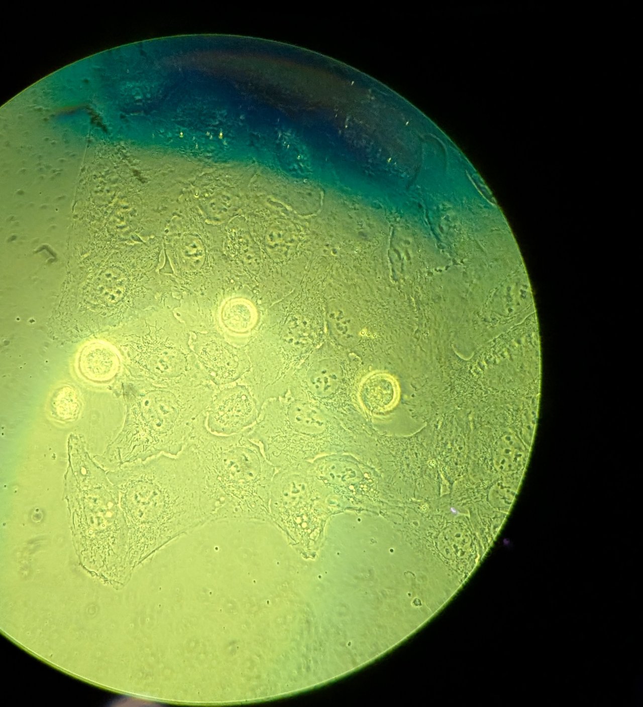
Close down the field stop unitl it is fully closed. You will see something similar to the following in the eyepiece.
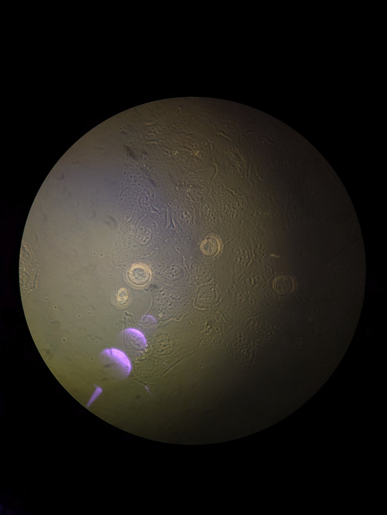
Step 4
Be careful in this step not to drive the condenser into the glass on the CO2 chamber!
Slowly adjust the height of the condenser until it is just above the glass on the CO2 chamber. Bring the edges of the field stop into focus using the height adjustment. You may need to switch between adjusting the height and adjusting the XY position of the condenser using the adjustment screws to find the edges.
Be patient; this part takes some time and practice.
Once the field stop is in focus, center it.
Step 5
Return the condenser tower to its original, upright position.
Set the microscope back to the side port light path and proceed to the next section.
Image the Cells in Fluorescence
This section assumes that the you have performed the steps in the last two sections. Most importantly, you have found the cells and they are in focus.
We will perform fluorescence imaging of mitochondria in this section. The cells have been modified to express StayGold fluorescent protein that is targeting the mitochondrial matrix. No staining is necessary.
Instructions
Step 0
In the Configuration Settings section of the Micro-Manager control panel, set the Channel to GFP (470 nm).
It’s OK to leave the Transmitted Light Intensity at a non-zero value because the transillumination lamp will not turn on when the GFP channel is active.
Adjust the 470 nm Intensity to some non-zero value.
Step 1
Click Live. You should see:
- a fluorescence image of the mitochondria in the
Livepanel, and - blue light coming from the objective. (There is no need to look directly over top the sample; you should not do this anyway for eye safety reasons.)

Step 2
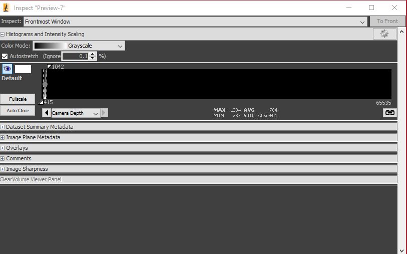
Check the Image Inspector window, which displays a histogram of all the pixel values.
In the example below, you can see that the histogram lies near the bottom of the range of pixel values (0 - 65535). The minimum is 237 analog-to-digital units (ADU) and the maximum is 1334 ADU, with an average of 704 ADU.
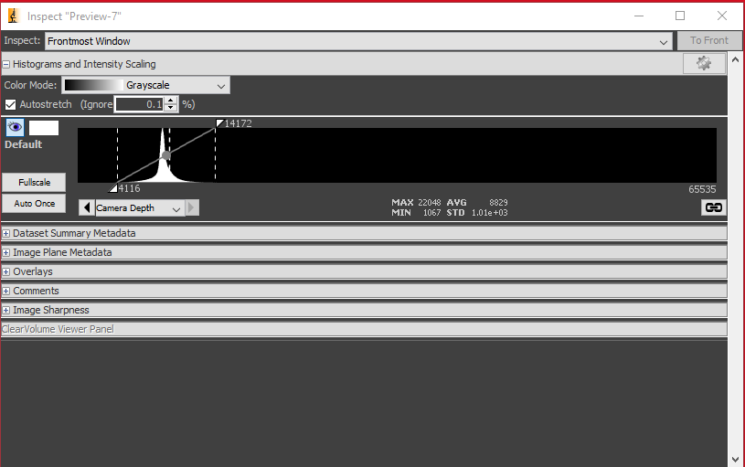
Step 3
Increase either the exposure time or the LED intensity. You should see the histogram shift to the right like below.
The live image should appear less noisy as well, which corresponds to it having higher signal-to-noise ratio (SNR).
Try to adjust the intensity and the exposure time until the histogram is as far to the right of the range as possible without saturating any pixels.
Step 4
Select the Multi-D Acq. button in the Micro-Manager control panel. This will open the Multi-Dimensional Acquisition window as shown below.
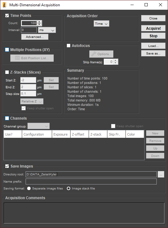
Step 5: Take a Time-Series Acquisition
Ensure that Time Points is checked and that Multiple Positions, Z-Stacks, and Channels are unchecked. Set the count to 100 and the interval to zero. (Image as fast as possible.)
For the directory root, select D:\DATA_Zeiss\<your name>\<YYYYMMDD_experiment_name>. For the name prefix, enter something short and descriptive, such as U2OS_Staygold.
Ensure that Image stack file is selected, and enter any additional metadata you wish to save in the Acquistion Comments.
Click Acquire!
You can review the images after they have been acquired.
Step 6: Z-Stack Acquisition
Find a suitable focal plane for your cells to serve as the center slice of the Z-stack.
In the Multi-D. Acquisition window, ensure that Z-Stacks (Slices) is checked and that Time Points, Multiple Positions, and Channels are unchecked.
Check the Keep Shutter Open checkbox to avoid rapidly turning the light on and off during the acquisition. Set the Start Z and End Z values to -1 and 1, respectively. Set the Step size to 0.1.
You can keep the directory root and prefix values the same as before. Micro-Manager will append a number to the end of the folder to ensure that any existing data is not overwritten.
Click Acquire to launch the acquisition.
Step 7
When you have finished, you may close Micro-Manager. The hardware is turned off in the reverse order that it was turned on.
Step 8
Push back the condenser tower. Remove the sample and insert from the stage. Clean the objective with lens cleaning tissue and ethanol as instructed.
Discussion
Imaging Parameters Optimization
If all you wanted to do was to maximize the signal-to-noise ratio (SNR) of your images, then you would increase the exposure time and/or light intensity until the histogram was as close as possible to the upper limit of its domain without saturating any pixels.
But what if the intensity is maxed out and you still have room left in the histogram to improve the SNR? You could increase the exposure time still further. But, as a result, doing so would decrease your frame rate. If you also needed to image fast dynamics within the cell, and these required a minimum frame rate, then there would be an upper limit to the value for the exposure time that you could set. Beyond this value, you would not have a high enough frame rate to see the thing that you would like to see; it would be blurred out.
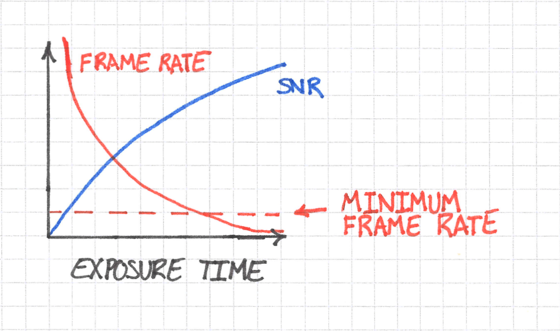
Ultimately this means that you must sacrifice some SNR to obtain a sufficient temporal resolution. We can visualize the problem like this:
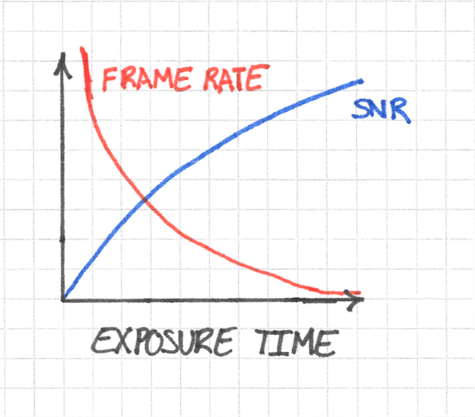
Do not worry too much about the exact shapes of the curves in the sketch above; what’s important are the trends. SNR increases with exposure time, whereas frame rate decreases. The dynamics that you want to see impose a requirement on the minimum frame rate at which you can image. You can imagine this minimum as follows:
But the minimum frame rate also imposes a maximum on the exposure time. This value is just the vertical line through the point of intersection of the frame rate curve and its minimum required value.
Taking this logic one step further, the maximum exposure time also imposes a maximum achieveable SNR, so in the end we have something like this:
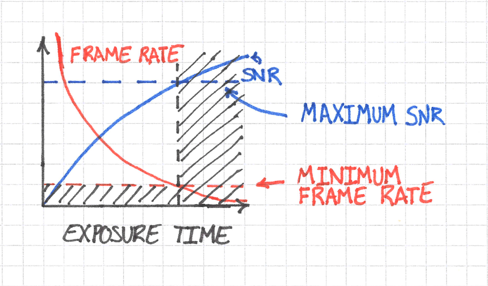
The frame rate requirement ends up reducing the parameter space of exposure time and, subsequently, the maximum achieveable SNR.
We have finally arrived at an optimization problem: given the frame rate requirement, what exposure time maximizes SNR?
The answer in this case is straightforward: it’s the exposure time where the frame rate is just fast enough to see the dynamics that you are after.
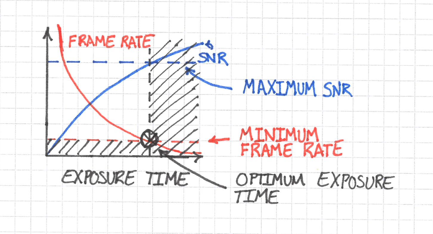
You can of course image at shorter exposure times, but then your SNR will suffer.
I think it’s worth making explicit the logic in this example because it’s central to how one should think about performing imaging experiments:
- First we identified our requirements (the timescale of the cell’s dynamics).
- Next, we turned the problem into an optimization problem. We decided to maximize SNR (a quality of the images) by tuning the exposure time (a property of the microscope).
- We then solved for the exposure time that maximized the SNR.
But What Parameter Values should I Choose?
The above discussion is fine from a theoretical perspective, but you’re probably wondering how to set the actual value of the exposure time when at the microscope. Or, for that matter, how do you actually set any microscope property? After all, you’re not going to have the nice simple plots that I drew above when making your decision. Rather, you’re going to have only what you see in the images.
This is where imaging becomes a bit more art than science. Regardless, we can still approach the problem systematically.
Feasibility
First, I recommend that you think broadly about what you’re imaging to set some bounds. A cell biologist looks at organelles, and from experience we know that these move on the order of milliseconds to tens of seconds. A developmental biologist studying embryo development, on the other hand, cares about timescales that are probably more on the range of hours to days. In these cases, you can conclude that frame rates are probably going to be somewhere between 1 and 10,000 frames per second (fps) for the cell biologist and much slower for the developmental biologist.
With bounds established, you should next consider your requirements and constraints. CMOS cameras have exposure times anywhere between fractions of a millisecond to tens of seconds. If you want to study something faster than the camera can image, then you’ll need a different approach entirely.
Parameter Tuning
After having decided that your experiment is at least feasible, you’ll need to develop a sense for what makes a “good” image dataset.
One quality of good images is that they have high SNR. But how do you estimate SNR? By using the image histograms. As previously mentioned, a good SNR means the center of the distribution of pixel values in the histogram is as close as possible to its upper limit without saturating pixels. But keep in mind that this is not the same as measuring the SNR directly. So you will have to develop a feel for how to estimate image qualities indirectly from images and their histograms.
Another quality of good images is that they satisfy your requirements. Do you image fast enough to see the thing that you want to study? How do you know what frame rate is required if you haven’t looked yet? Here pilot experiments can help. You can try a range of exposure times and frame intervals on test samples and see roughly what range of values works. You may not arrive at exact values, but you can at least establish a rough order of magnitude.
Back of the envelope calculations help to pinpoint ranges of parameter values in some scenarios. For example, in tracking experiments, if you know the density of particles and their diffusion constants, then you can work out what frame rate is necessary to capture a certain number of frames before a collision occurs with another particle.
What Else can I Adjust in my Experiments?
It’s not only microscope parameters that can be tuned. Signal-to-background ratio (SBR), which I discuss in the next section, can be improved through better sample preparation or a change of microscope. A switch from widefield to confocal microscope can help in this scenario in particular. Try to identify what aspect of the experiment is preventing you from answering your hypotheses, and then look at what can be changed to make it possible.
What about Photobleaching, Phototoxicity, Spatial Resolution, and Signal-to-Background Ratio?
I deliberately left these out of the discussion above to keep it simple, but they need to be considered as well. Phototoxicity and photobleaching ultimately limit the laser intensity (which in turn limits the SNR) and the length of your experiments. You won’t be able to avoid these effects entirely.
Spatial resolution is harder to adjust through microscope parameters alone since it depends heavily on the microscopy method itself. Still, improving SNR does slightly improve spatial resolution, and choice of microscope is just as important as anything else when designing an imaging experiment. Likewise for signal-to-background ratio. Lightsheet microscopes have become so popular because they efficiently solve the issues relating to SBR.
The key is to establish the requirements for your experiments in terms of these qualities:
- spatial resolution
- temporal resolution
- SNR
- SBR
- phototoxicity
and these constraints:
- budget
- time available
- equipment available
- expertise
I’m going to say it again because it’s so important: without any requirements or constraints, there is no way of doing meaningful, quantitative experiments on a microscope because there is nothing to optimize.
Polyhedra of Democracy
You might have heard of the “triangle of frustration”, “pyramid of compromise,” or similar terms. One such example looks like this (source):
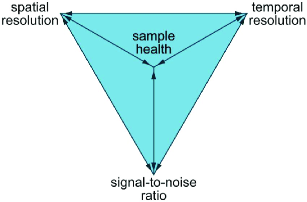
The idea here is that you can move about within the pyramid by adjusting imaging parameters, the microscopy method, the sample preparation protocol, and more. In doing so, you improve on one of the qualities at the vertexes of the pyramid but necessarily sacrifice something at the other vertexes. Improving spatial resolution, for example, might mean decreasing temporal resolution and cell health.
Again, it’s very hard to put the imaging problem on firm, algorithmic grounds with definite data. This is partly because we can’t measure everything we need to (how do you quantify phototoxicity?), partly because it’s not always clear what makes for an optimum set of parameter values. Still, these concepts help you navigate the challenges inherent in optimizing your imaging experiments by
- making clear what the tradeoffs are, and
- helping design pilot experiments that help narrow in on the right range of microscope parameter values.
Questions
-
True or false: Köhler illumination produces flat illumination, i.e. the light intensity does not vary across the sample.
-
Assume you would like to take a time series acquisition of live cells. You use Micro-Manager and configure a Multi-Dimensional Acquisition with 50 ms exposure time, 10 frames, and 0 time interval between frames. True or false: the total acquisition time is 500 ms. (Hint: what is the readout time for the Photometrics Prime camera?)
-
True or false: the value of a pixel depends only on the rate of photons hitting it.
-
Why do we avoid saturating the pixels when imaging? (A pixel is saturated when its value is equal to its maximum value. For a 16 bit camera, this value is 2^16 - 1 = 65535.)
Image Acquisition
In this chapter we begin construction of a custom-built microscope for epifluorescence and transillumination imaging of cell culture samples.
We begin by explaining the basic components of a microscope and their layout. Then, we start the practical work by interfacing our microscope’s camera with the computer, installing the necessary drivers and capture software. As you will see, a working camera will be essential for aligning the microscope’s optical components.
Following this, we assemble our camera and tube lens into a simple, fixed focal length imaging system for imaging far away objects. We will align the camera and lens such that objects at infinity1 will be imaged onto the camera.
Finally, we set up Micro-Manager to control our camera. Using Micro-Manager will allow us to design and execute complex microscopy acquisitions that we otherwise could not do with the camera’s capture software.
-
The meaning of this phrase will be explained later in this chapter. For now, you can think of it as meaning objects that are far away. ↩
Set up the Camera
We start construction of the microscope by installing the camera software and making sure that it works correctly.
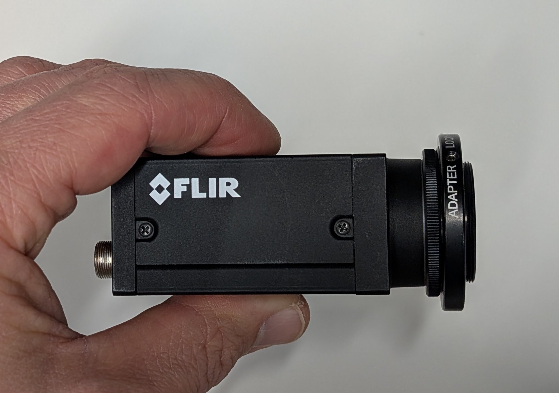
The camera used in this course is a Flir Grasshopper GS3-U3-51S5M. It is one of several small form factor cameras that are often referred to as industrial CMOS cameras in the literature. Industrial CMOS cameras are relatively cheap and compatible with fluorescence microscopes, but their noise characteristics and sensitivities are worse than more expensive scientific CMOS, or sCMOS, cameras. While most of our research is done with sCMOS camers, industrial CMOS cameras are still sufficient for applications in basic fluorescence microscopy.
Install the Drivers and Capture Software
To begin, we will install Flir’s Spinnaker software that includes the necessary camera drivers and the SpinView capture software. For reasons that will become apparent in a later section, you must install version 2.3.0.77.
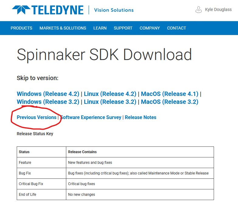
Navigate to https://www.teledynevisionsolutions.com/products/spinnaker-sdk in your web browser and select the Download button. Product software pages change frequently, so if the page has changed since this was written, you will need to search for the Spinnaker SDK (software developer kit) and find it on your own.
You will be asked to create an account or sign in after clicking the Download button. Go ahead and do so.
Once logged in, you will see a page that looks like the following. Be sure to select the link for previous versions!
Download the Windows version 2.3.0.77 installer. Unzip the file, and launch the installation with the x64 version of the installer1. When prompted, select Applicaton development, though Camera evaluation should work as well. There is no need to install the GigE camera driver2. Any other settings may be left with their default values.
Start Device Acquisition
After installation has finished, attach the camera to the PC with the blue USB cable and start the SpinView software. You will see a screen that looks like the following:
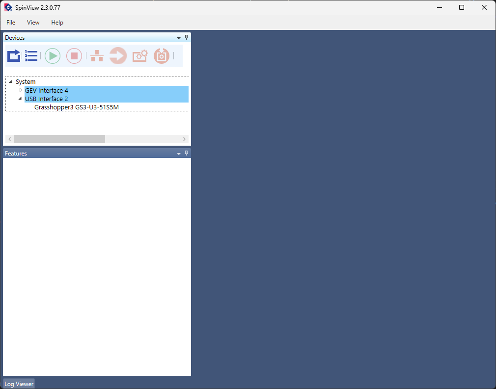
Confirm that the camera is recognized by the computer by finding it in the list of devices in the upper left panel of the screen. The camera used in this lab is a Grasshopper3 GS3-U3-51S5M. Select the camera in the list to enable its controls.
To acquire a live stream from the camera, click the green arrow at the top of the main image window. It should display the tooltip Start device acquisition when hovered over with the mouse. If all goes well, you should see a continuous stream of camera frames in the main window.
Verify the Camera Works as Expected
You will not be able to see anything resembling a real image in the live stream. (Do you know why this is?) Regardless, we can do a few basic sanity checks to ensure that the camera works as expected. Try the following:
- Take the cap off of the camera and wave it in front of a light. Verify that you see changes in brightness in the feed at the same time.
- Try to change the exposure time, frame rate, and gain. (Changing the frame rate requires changing more than one setting in the SpinView software.)
- Change the size of the region-of-interest (ROI) acquired by the camera.
- Change the format of the pixels from 8 to 16 bits.
Once you are satisfied that you understand the camera’s basic operation, we can move onto the next step.
-
The
x64version is for 64 bit operating systems. Thex86version is for 32 bit operating systems. Nearly all modern computers used in the lab are 64 bit. The most relevant difference between the two is that 32 bit operating systems are limited to using only 4 GB of memory, while 64 bit systems currently have no practical limit. There is however a theoretical limit of about 16 exabytes. ↩ -
GigE is an interface standard for transmitting image data over ethernet. ↩
Align the Camera and Tube Lens
In this section we build a fixed focal length camera that will serve as the base for building the rest of the microscope.
Parts List
Below is the parts list for this section of the basic training course. Note that some of the parts used in the course are now obsolete. In these cases the parts listed below are the closest current match to the obsolete parts.
| Part | Manf. Part No. | Quantity | URL |
|---|---|---|---|
| Camera | Grasshopper3 GS3-U3-51S5M | 1 | https://www.teledynevisionsolutions.com/en-150/products/grasshopper3-usb3/?model=GS3-U3-51S5M-C |
| Camera USB Cable | 1 | ||
| Cage Assembly Rod, 10“ Long, Ø6 mm | ER10 | 4 | https://www.thorlabs.com/thorproduct.cfm?partnumber=ER10 |
| 30 mm to 60 mm Cage Adapter, 0.5“ Thick | LCP33/M | 2 | https://www.thorlabs.com/thorproduct.cfm?partnumber=LCP33/M |
| Adapter with External SM1 Threads and Internal SM2 Threads | SM1A2 | 1 | https://www.thorlabs.com/thorproduct.cfm?partnumber=SM1A2 |
| Tube Lens, f = 200 mm, ARC: 350 - 700 nm, External M38 x 0.5 Threads | TTL200 | 1 | https://www.thorlabs.com/thorproduct.cfm?partnumber=TTL200 |
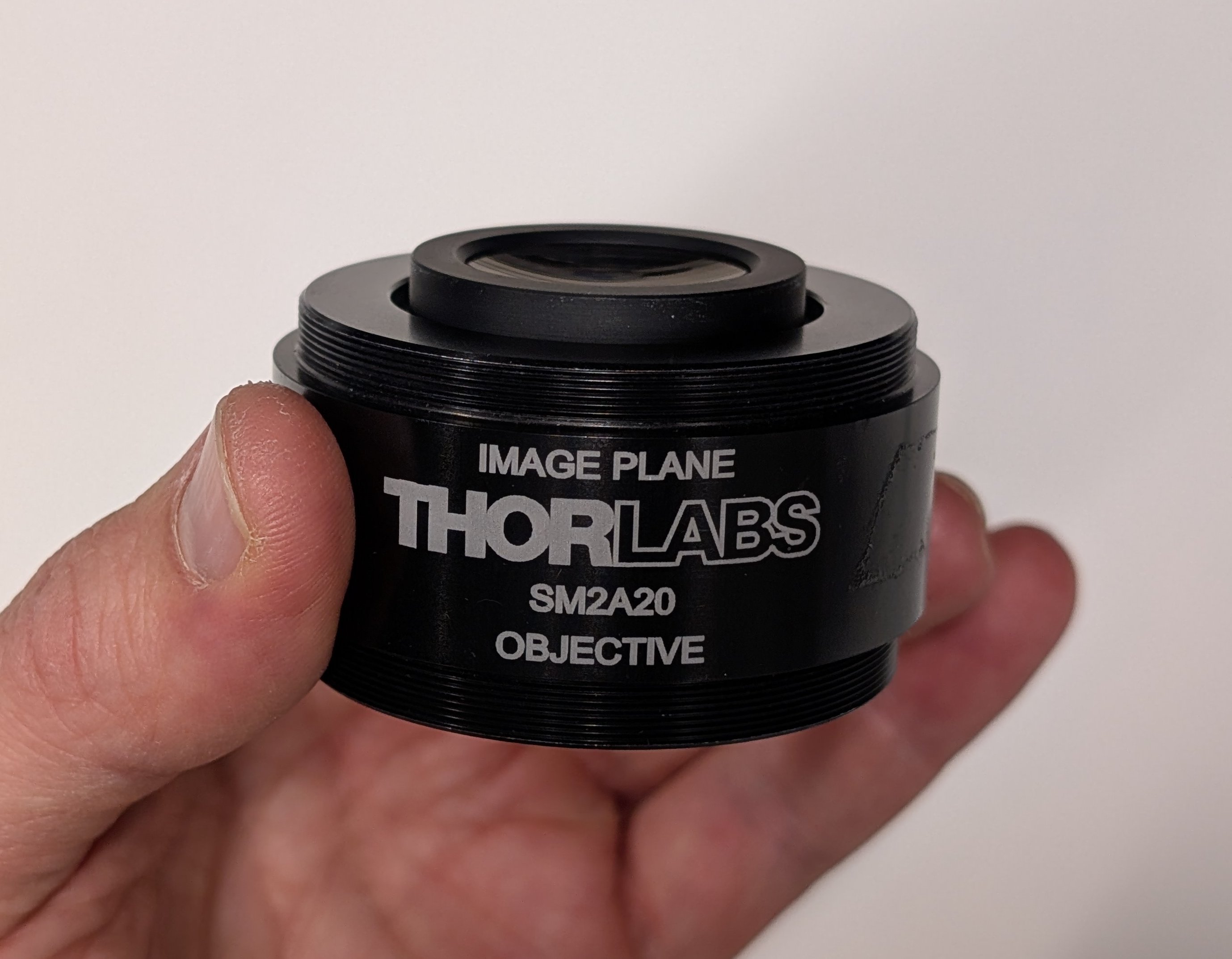
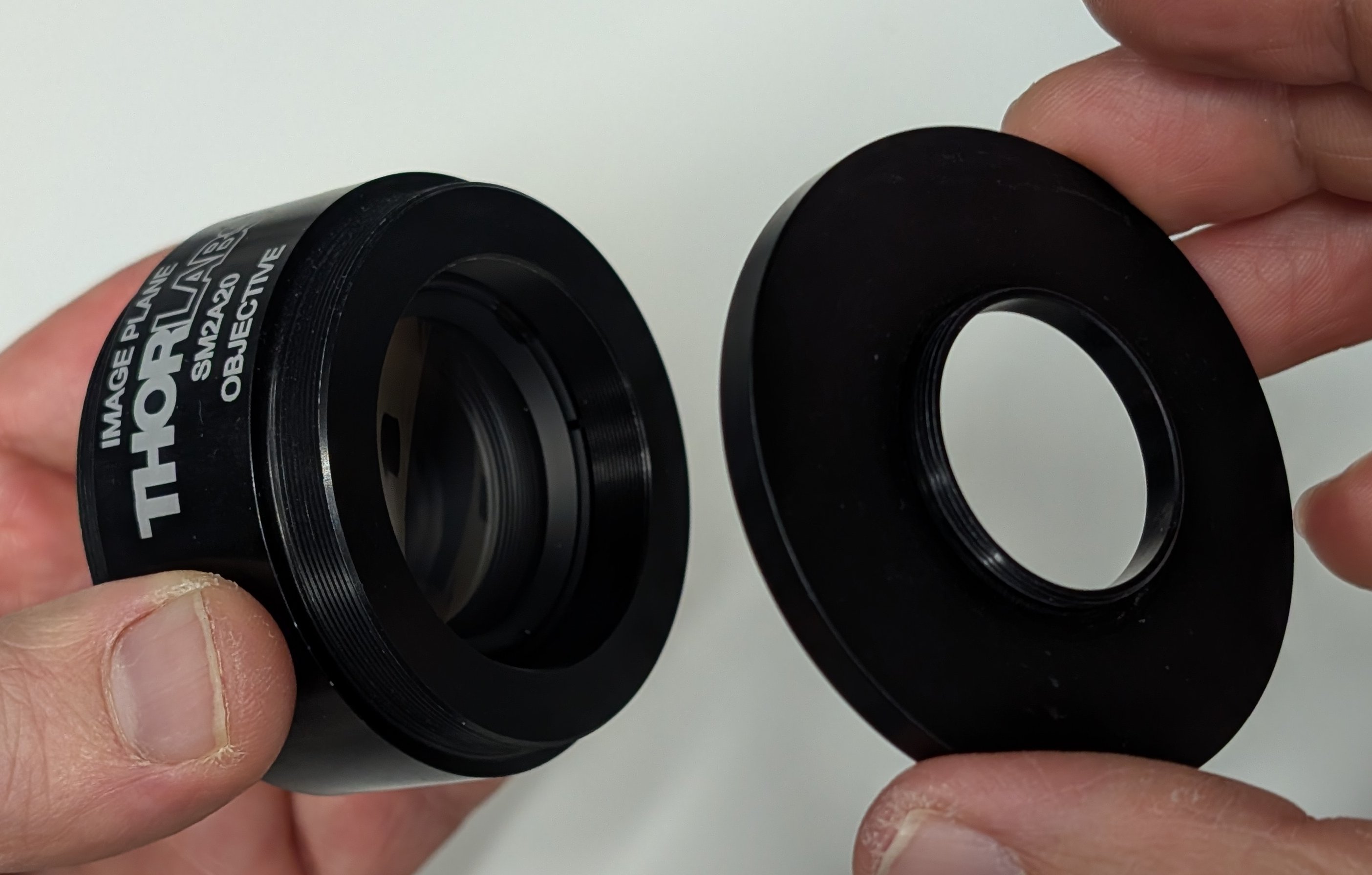
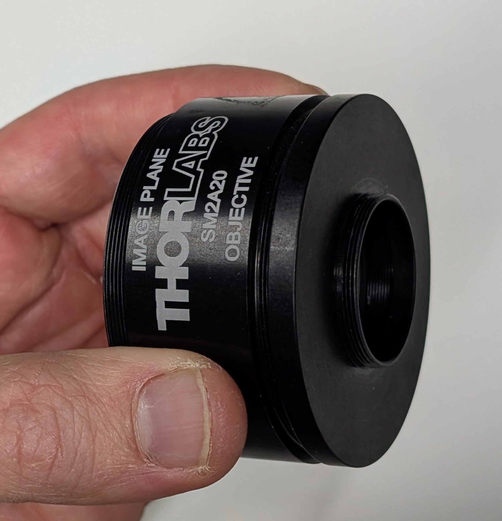
| Adapter with External SM2 Threads and Internal M38 x 0.5 Threads | SM2A20 | 1 | https://www.thorlabs.com/thorproduct.cfm?partnumber=SM2A20 |
| 60 mm Cage Plate, SM2 Threads, 0.5“ Thick, M4 Tap | LCP34/M | 1 | https://www.thorlabs.com/thorproduct.cfm?partnumber=LCP34/M |
| SM1 Quick-Release Adapter Set | SM1QA | 1 | https://www.thorlabs.com/thorproduct.cfm?partnumber=SM1QA |
| Adapter with External C-Mount Threads and External SM1 Threads, 3.2 mm Spacer | SM1A39 | 1 | https://www.thorlabs.com/thorproduct.cfm?partnumber=SM1A39 |
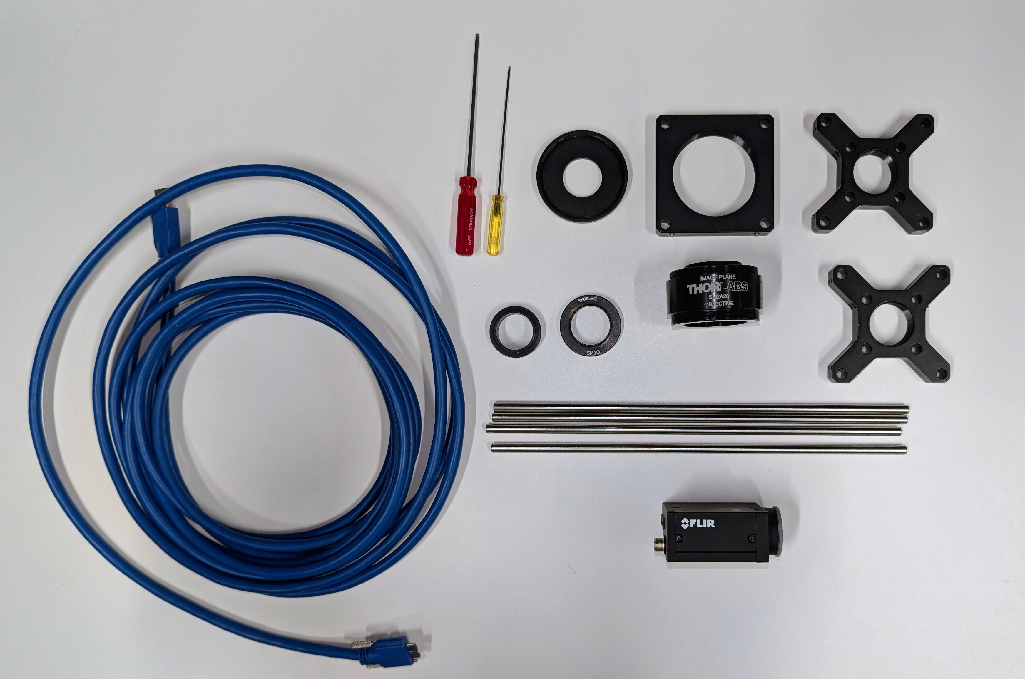
In addition, you will need 2 mm and 0.05“ Allen screwdrivers.
Instructions
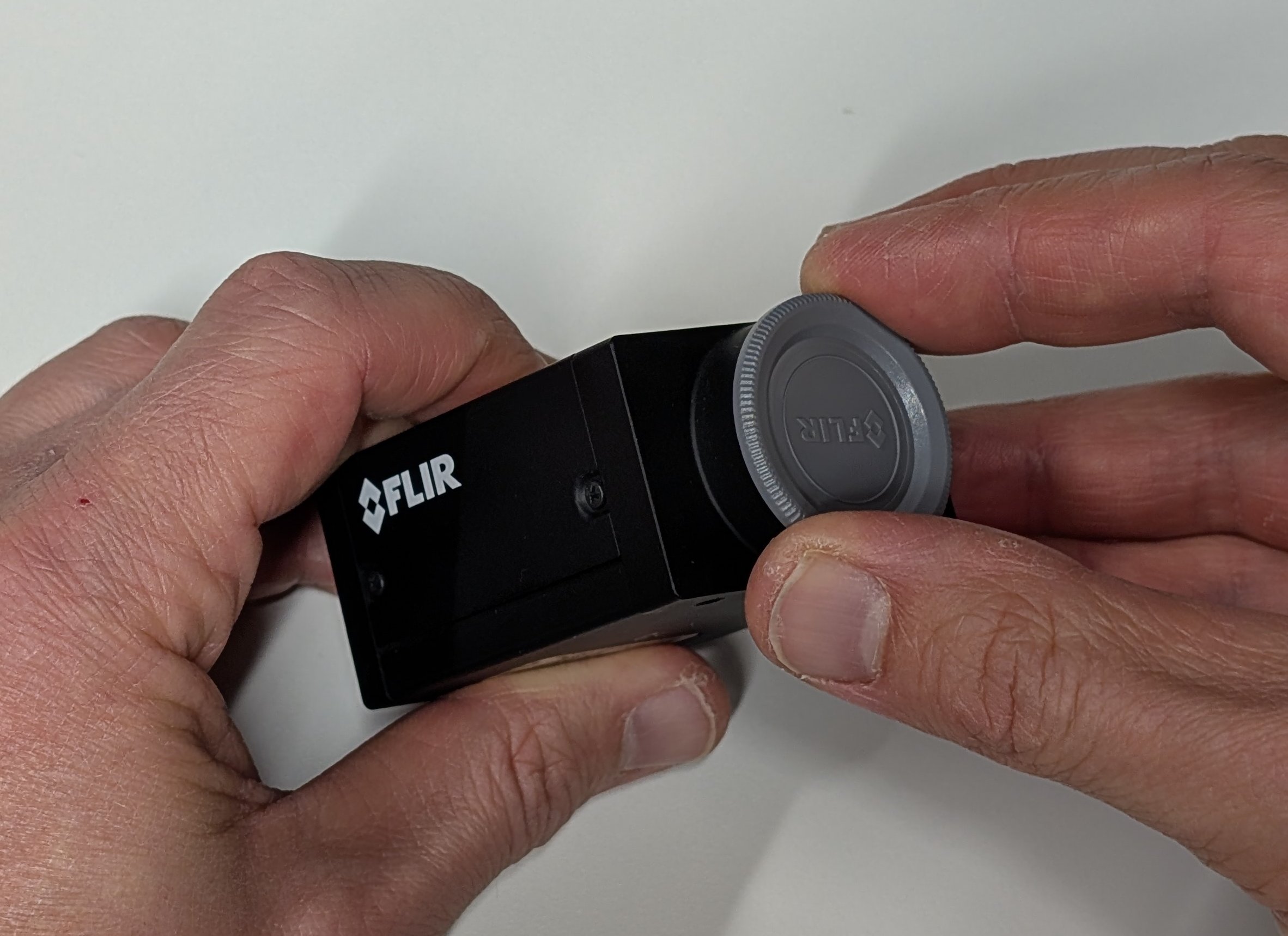
0
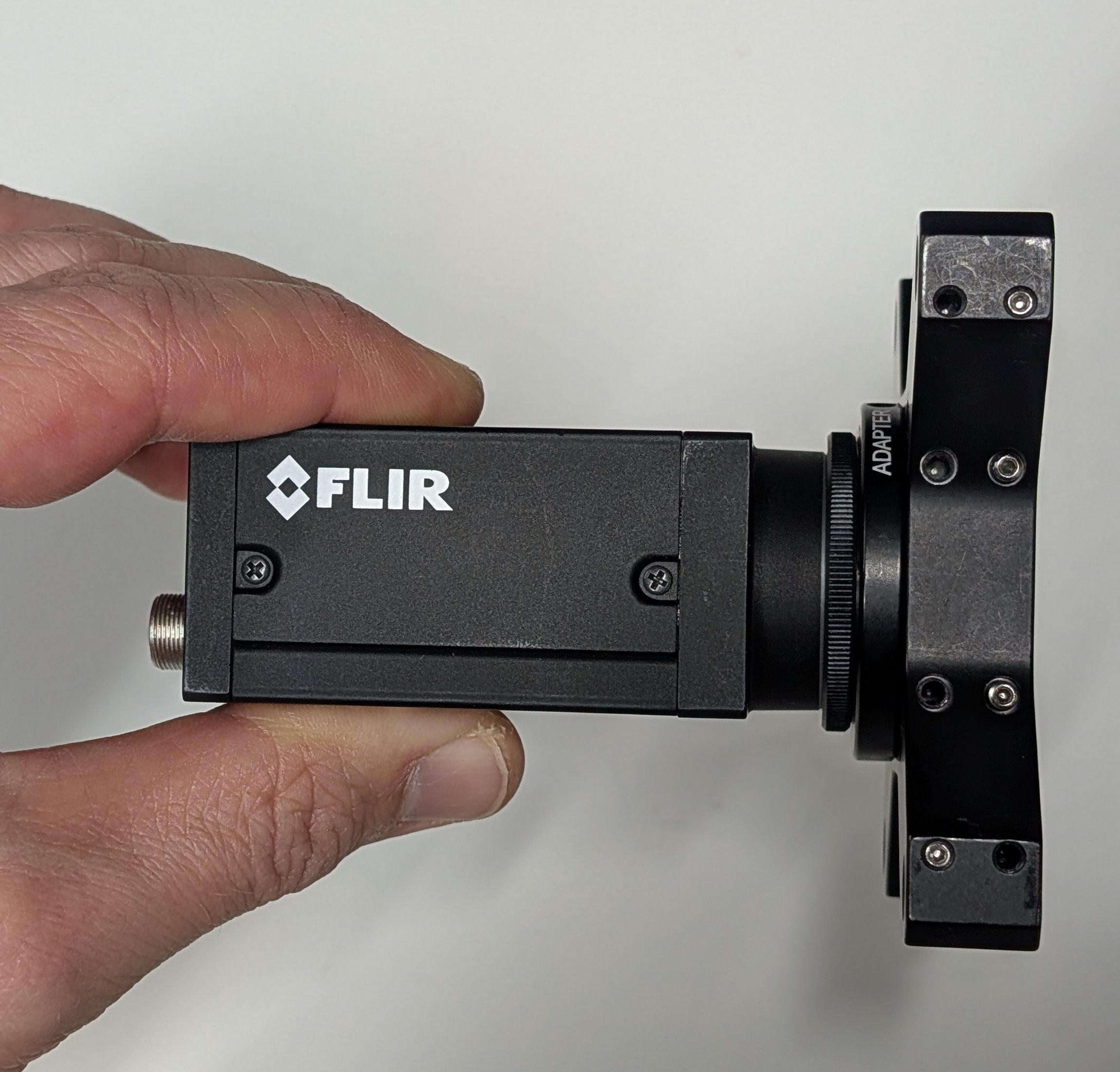
Remove the protective cap from the camera.
1
Attach the C-mount to SM1 external threads adapter to the camera.
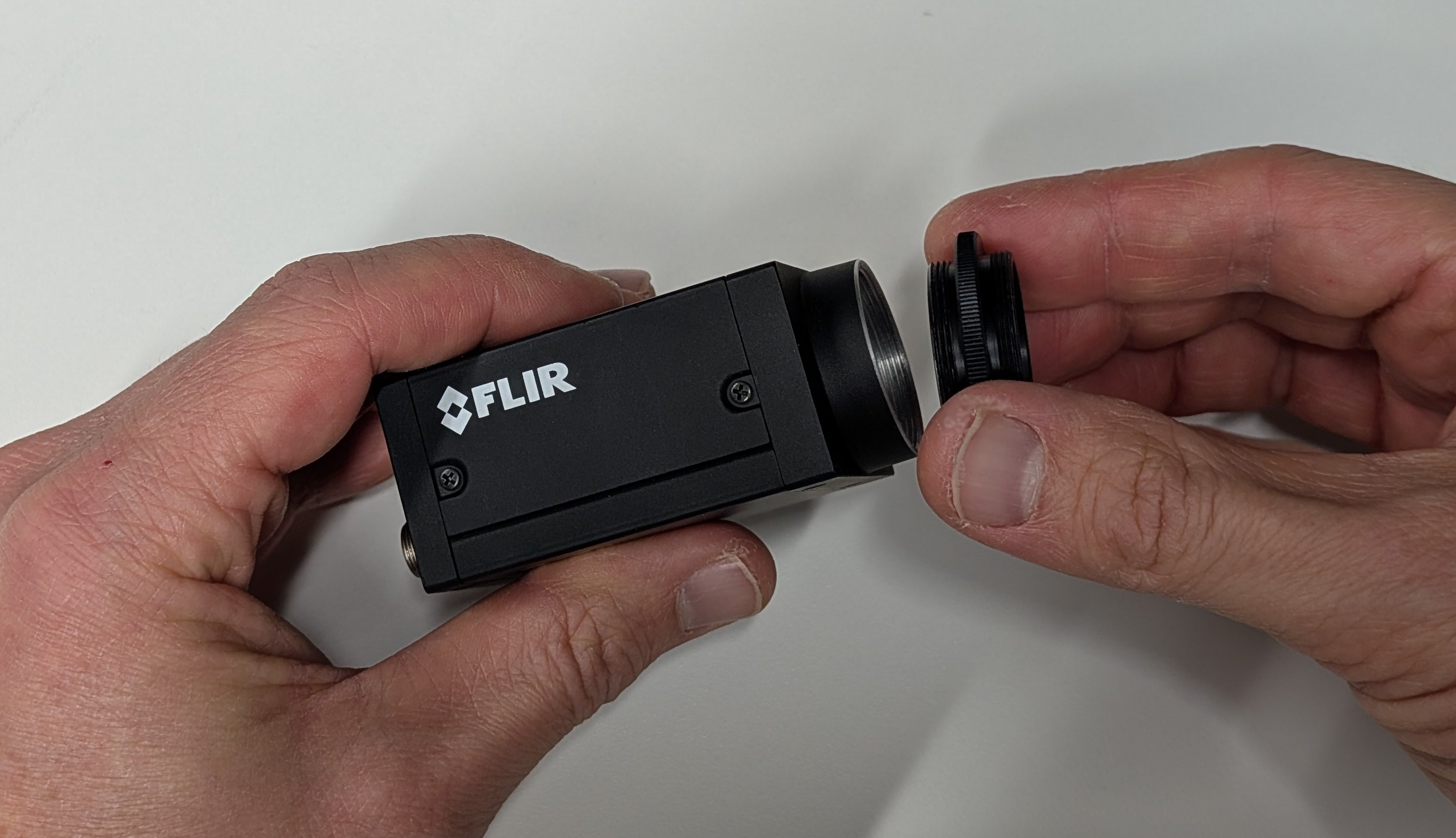
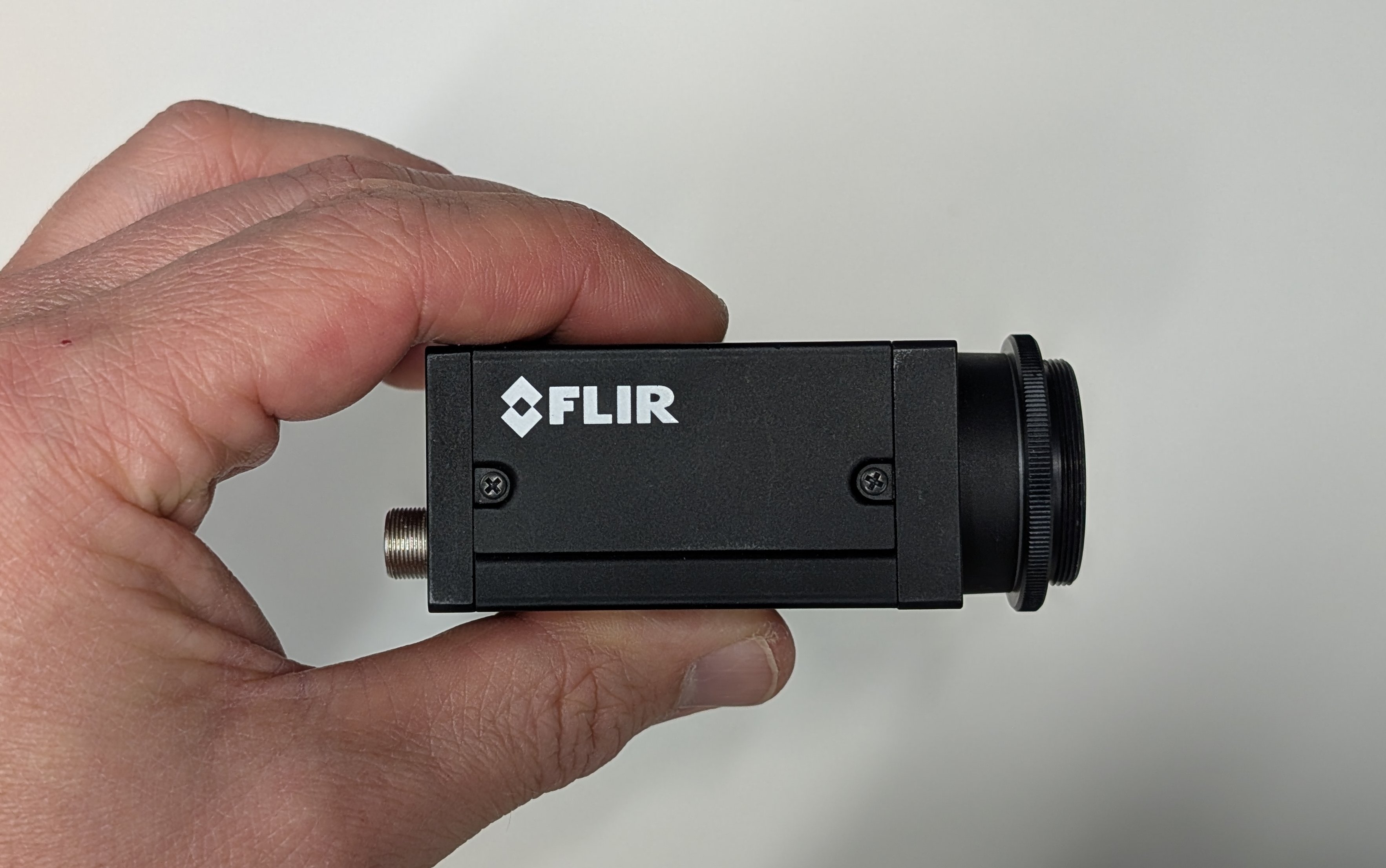
2
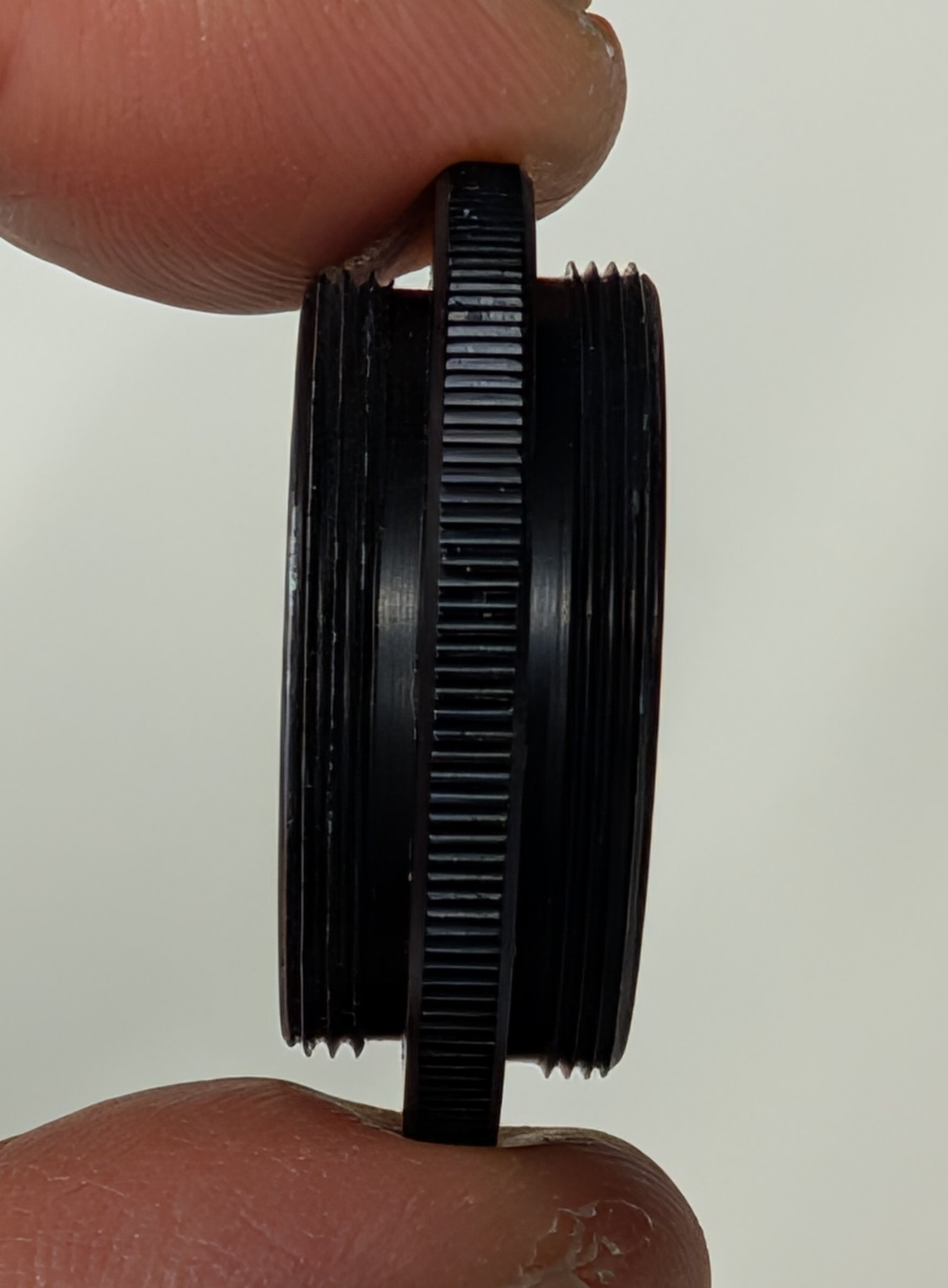
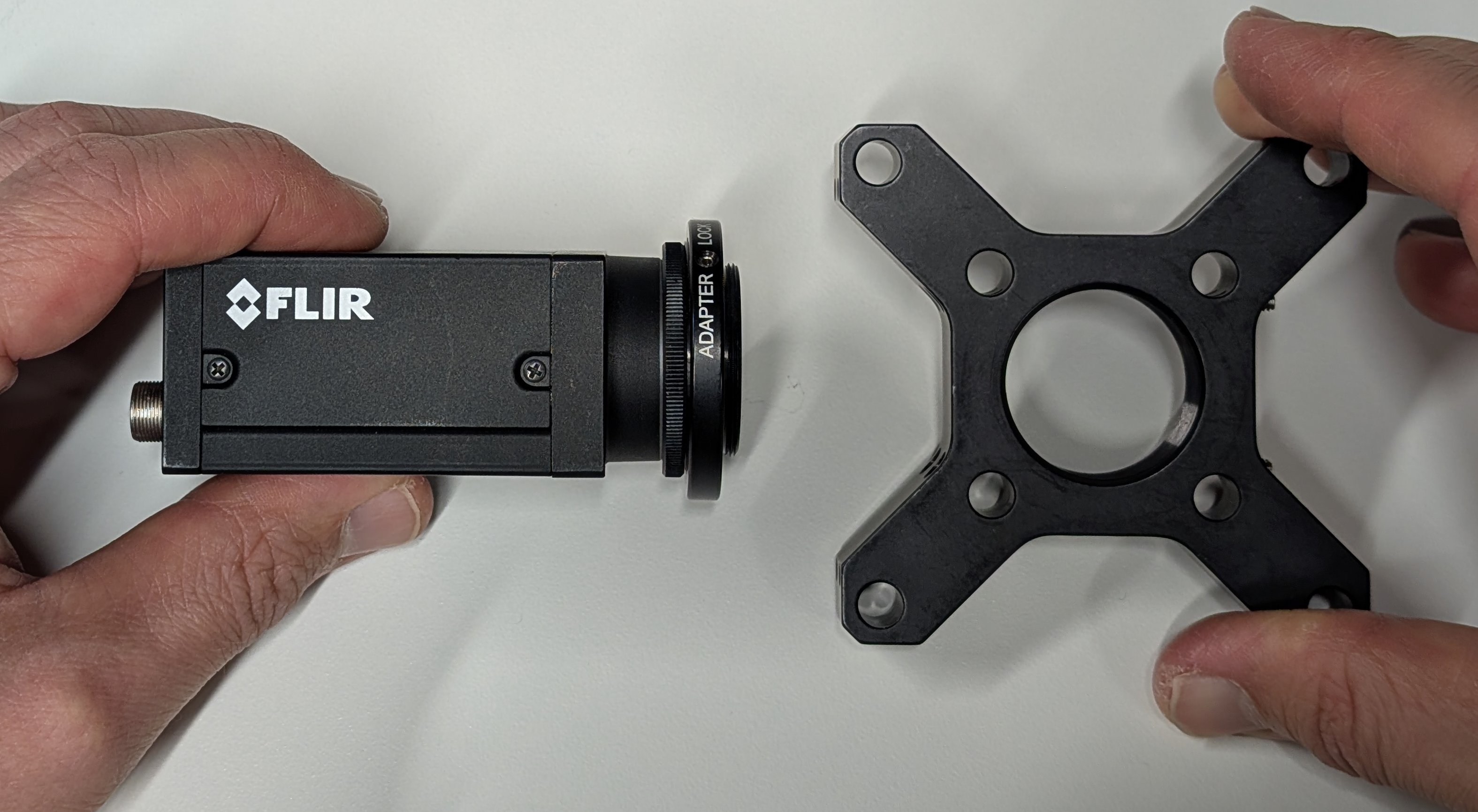
Attach the SM1 quick-release adapter set to the camera.
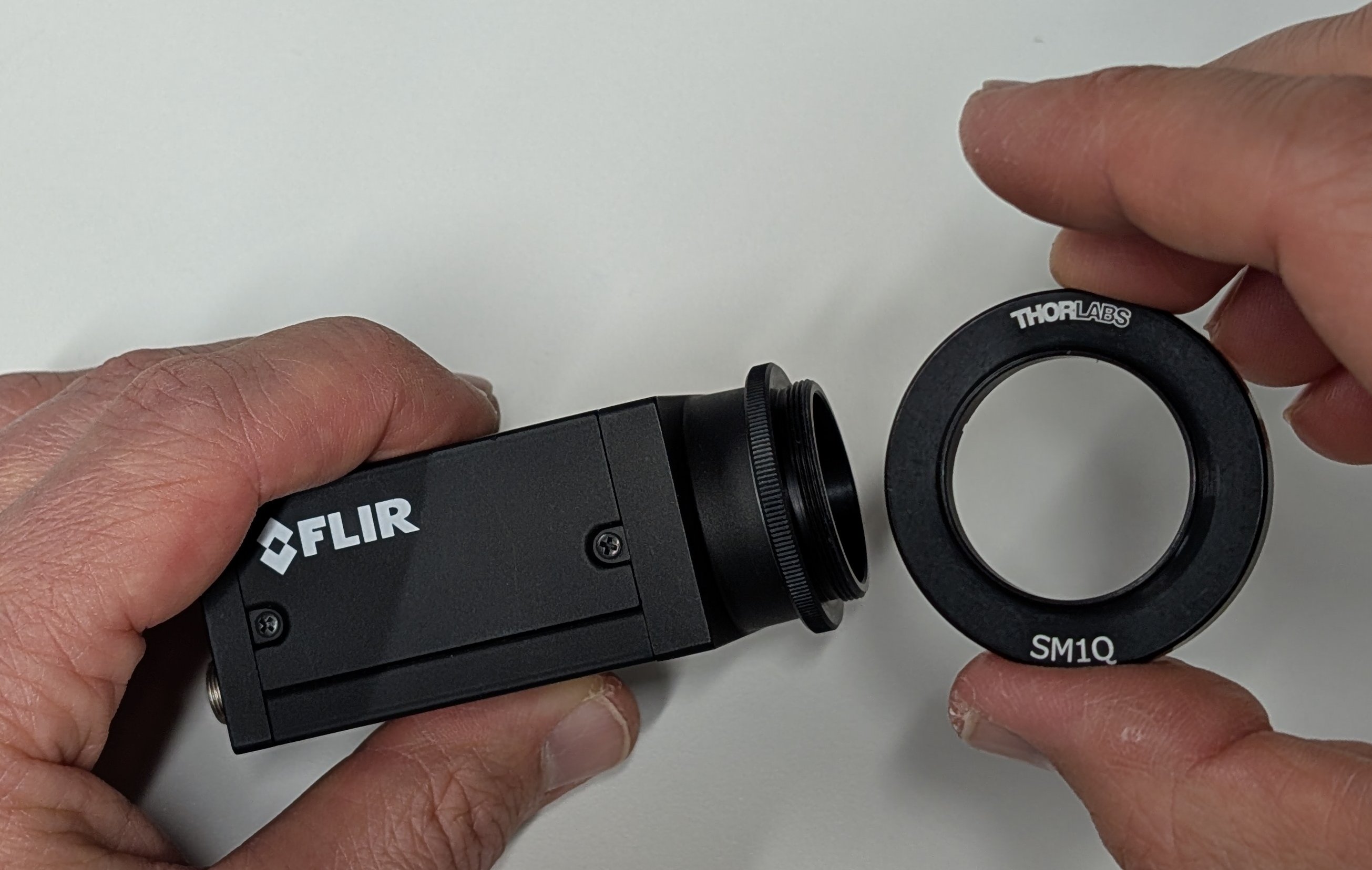
3
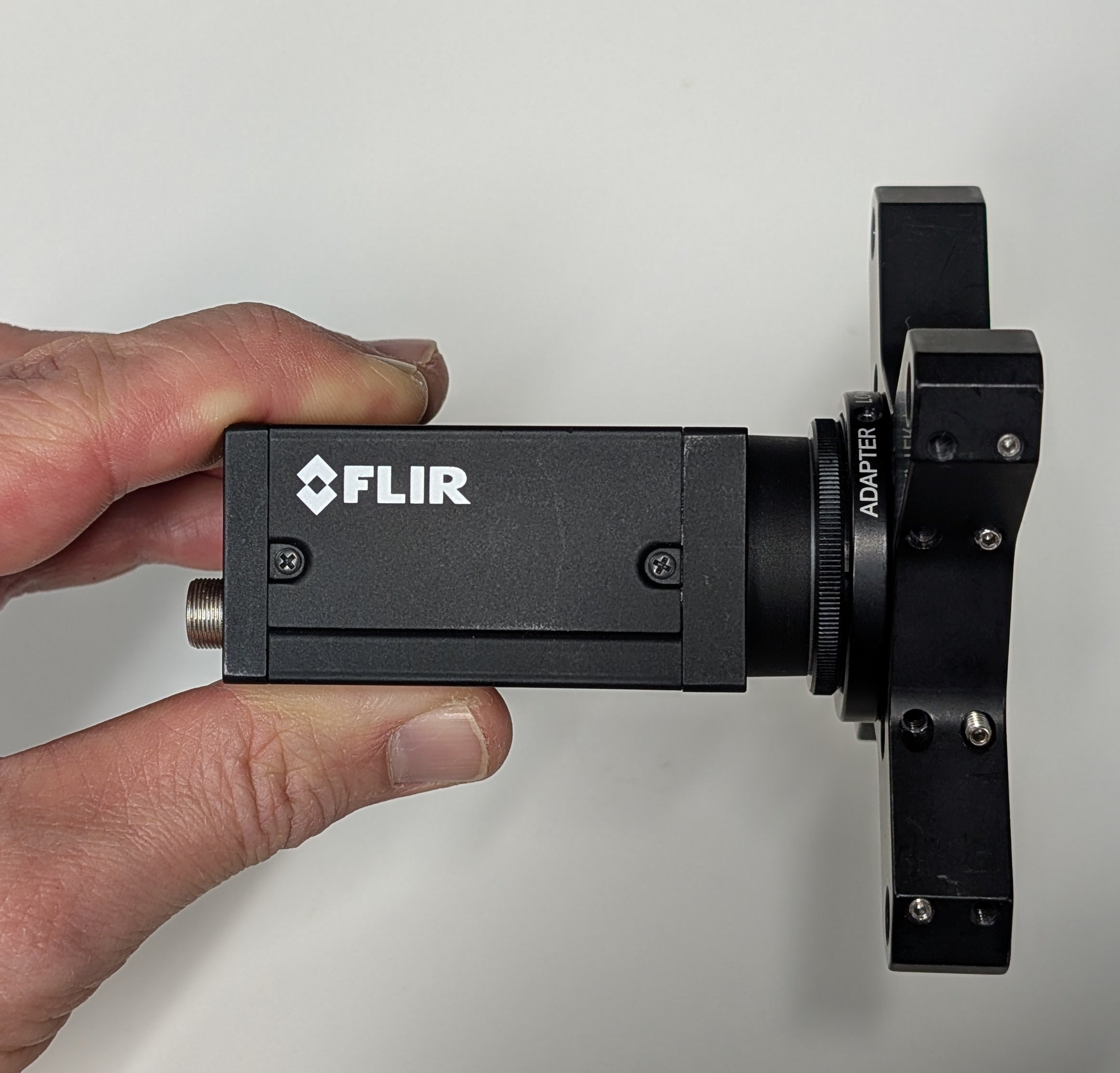
Attach one 30 mm to 60 mm cage adapter to the other end of the quick-release adapter via the SM1 threaded hole.
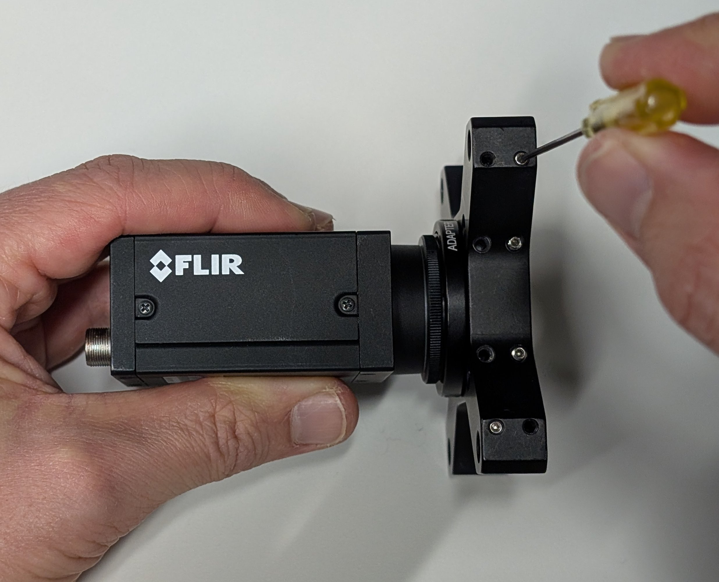
4
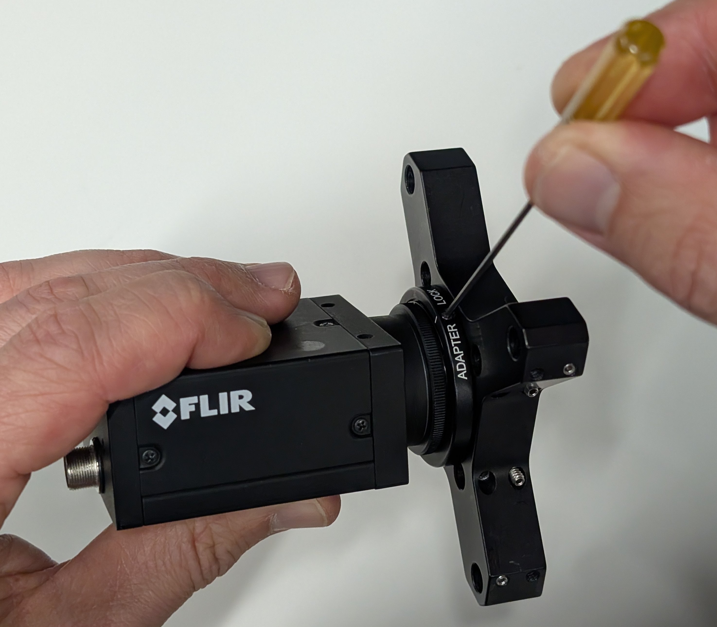
Use a 0.05“ hex driver to loosen the set screw on the quick-release adapter set. Rotate the camera until its body is aligned with the cage rod holes in the 30 mm to 60 mm cage adapter.
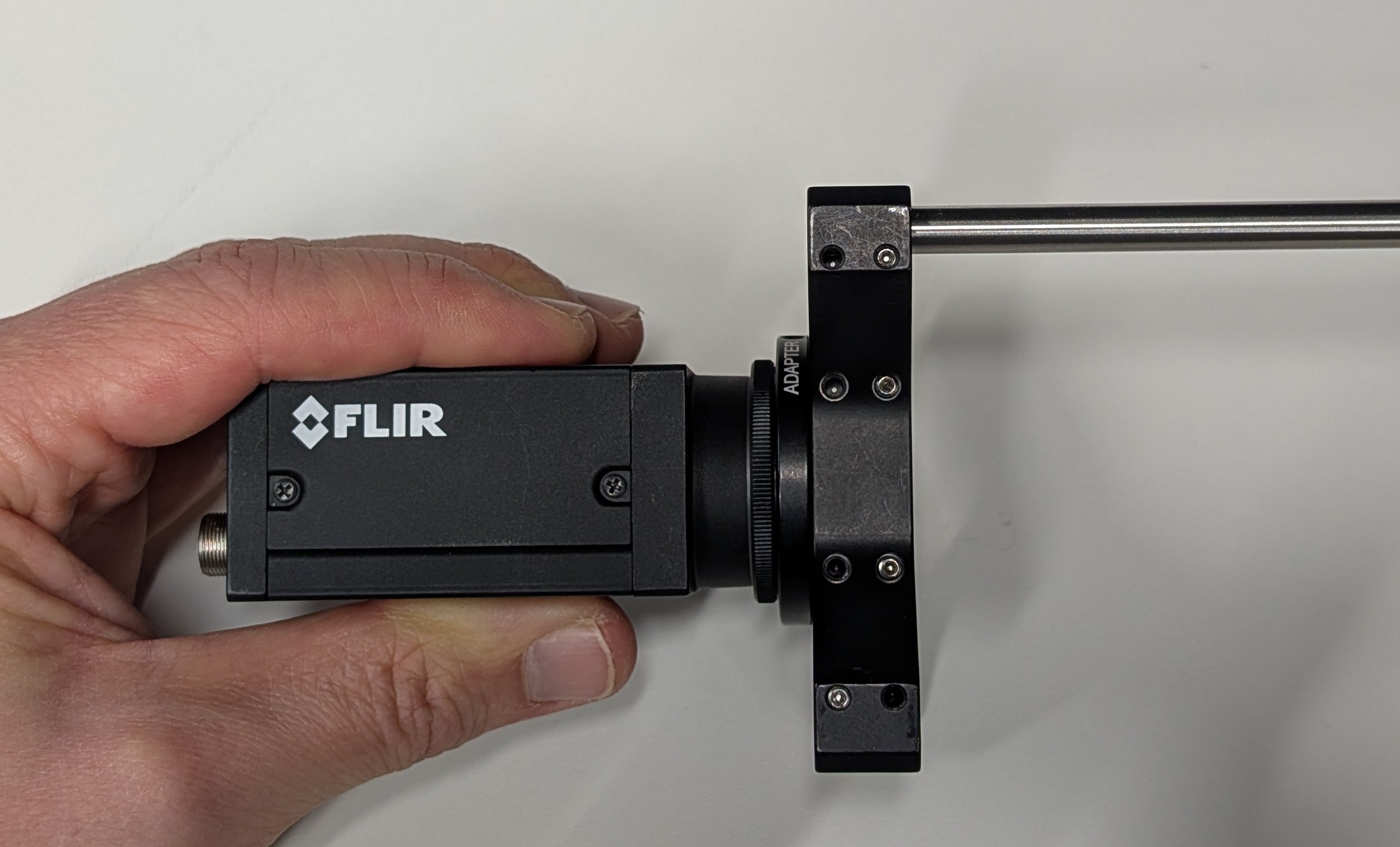
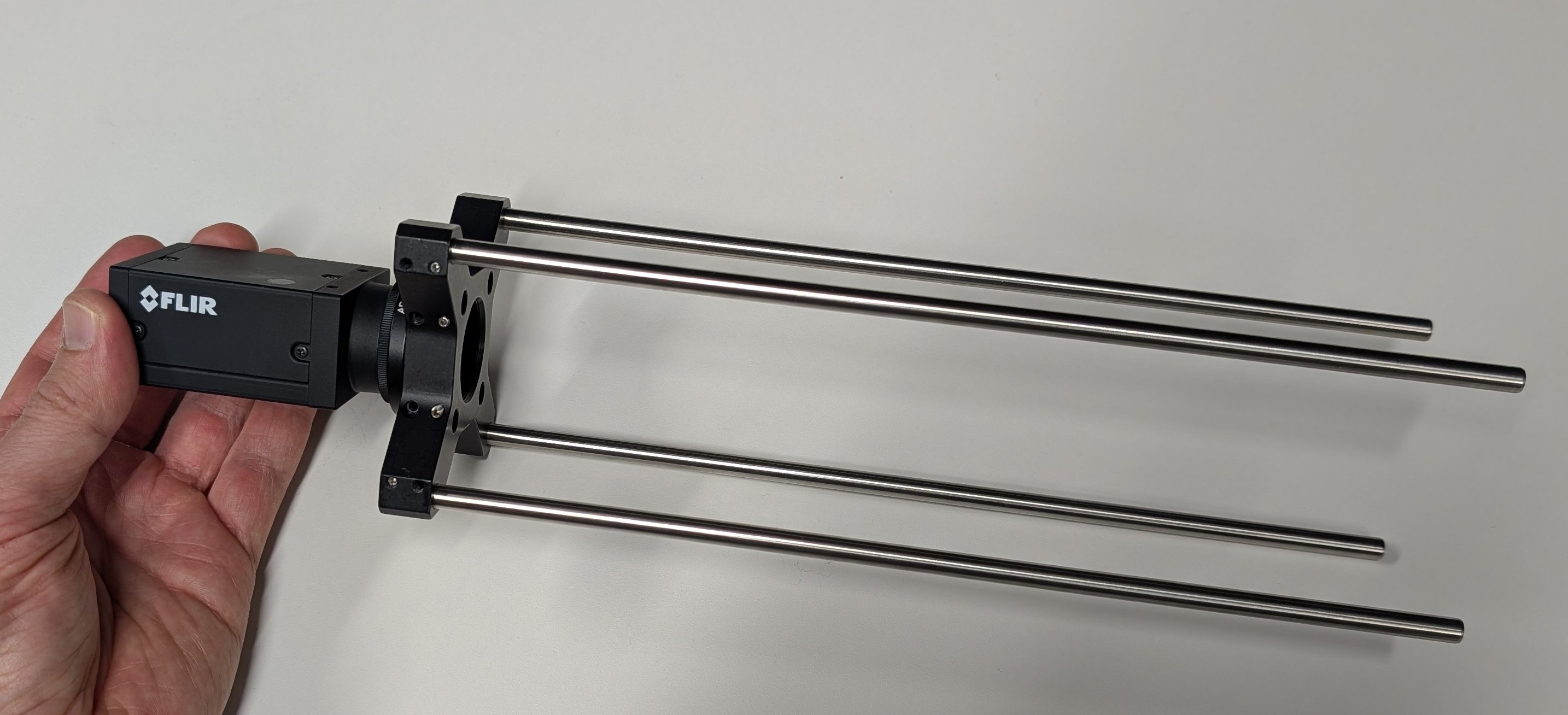
5
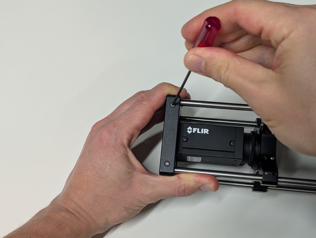
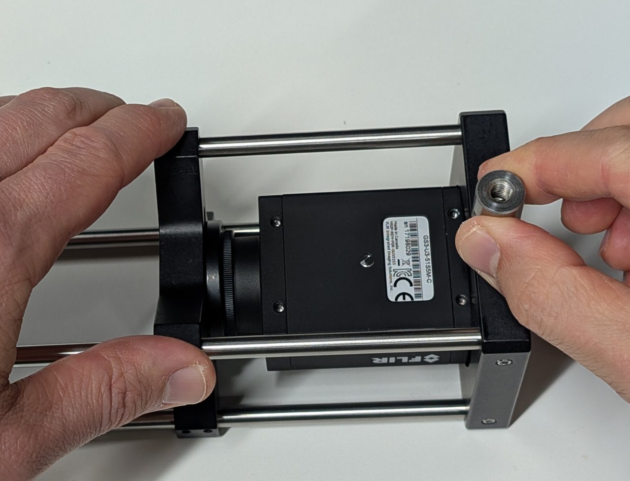
Loosen one of the set screws on the outer set of holes for the cage rods using a 0.05“ hex driver. Insert a cage rod and tighten the screw.
Repeat for all four cage rods.
For the older 30 mm to 60 mm cage adapters with 0.05“ set screws, it is OK if one of the two screws is missing.
6
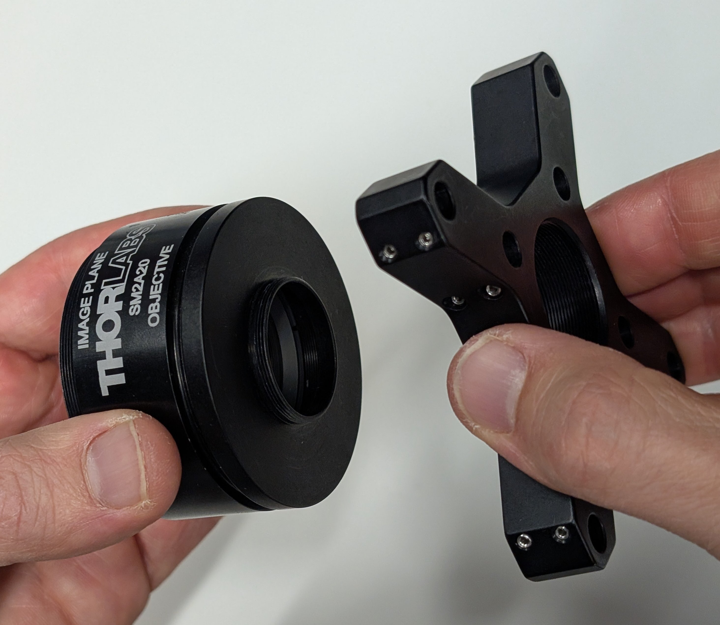
Thread the 200 mm tube lens into the SM2A20 tube lens holder if it is not already. Attach an externally threaded SM1 to interally threaded SM2 adapter to the tube lens holder on the side facing the objective.
7
Thread a 30 mm to 60 mm cage adapter onto the external SM1 threads of assembly from the previous step.
8
Slide the assembly from the previous step onto the other end of the cage rods and tighten the set screws so that the assembly does not slide along the rods.
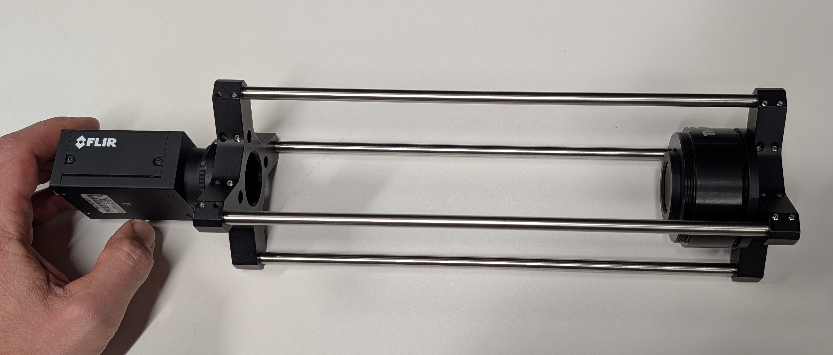
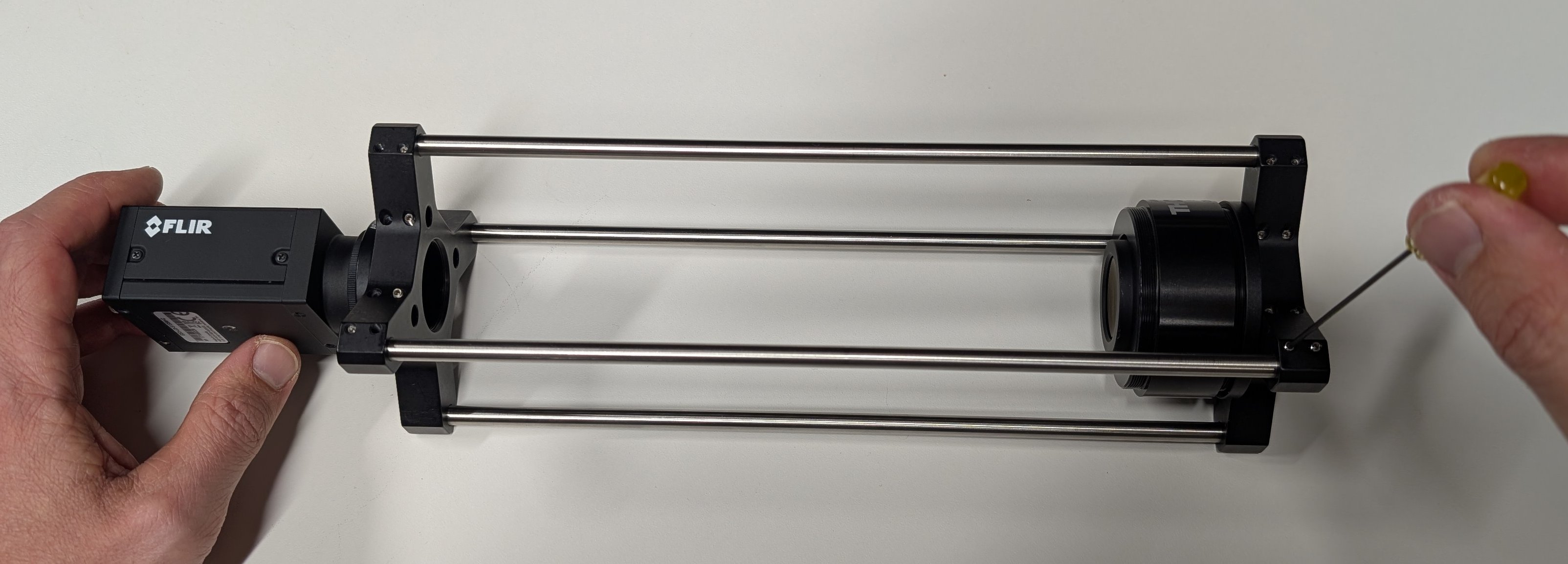
9
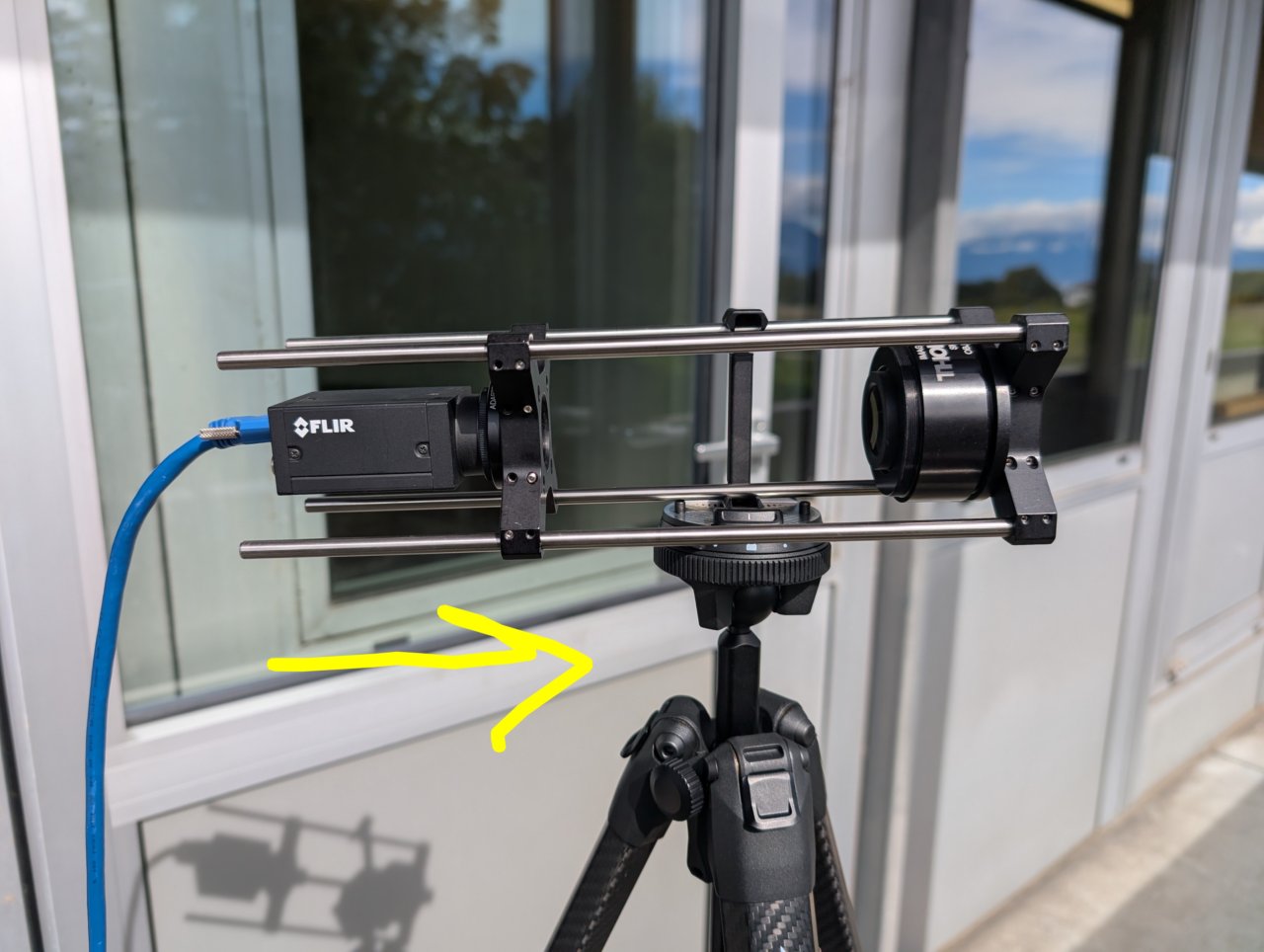
Plug in the camera and launch the SpinView software installed in the previous page. Take the lens assembly and PC to a room with a window with a view of far away objects, e.g. clouds or mountains. Start a live image feed and adjust the settings so that the image is not saturated.
One example for how to do this is illustrated below. It is not the only way.
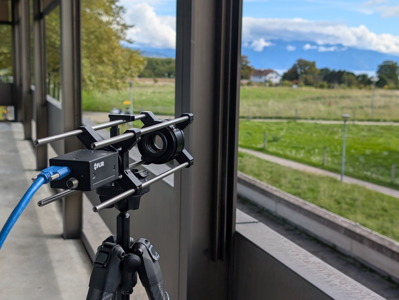
10
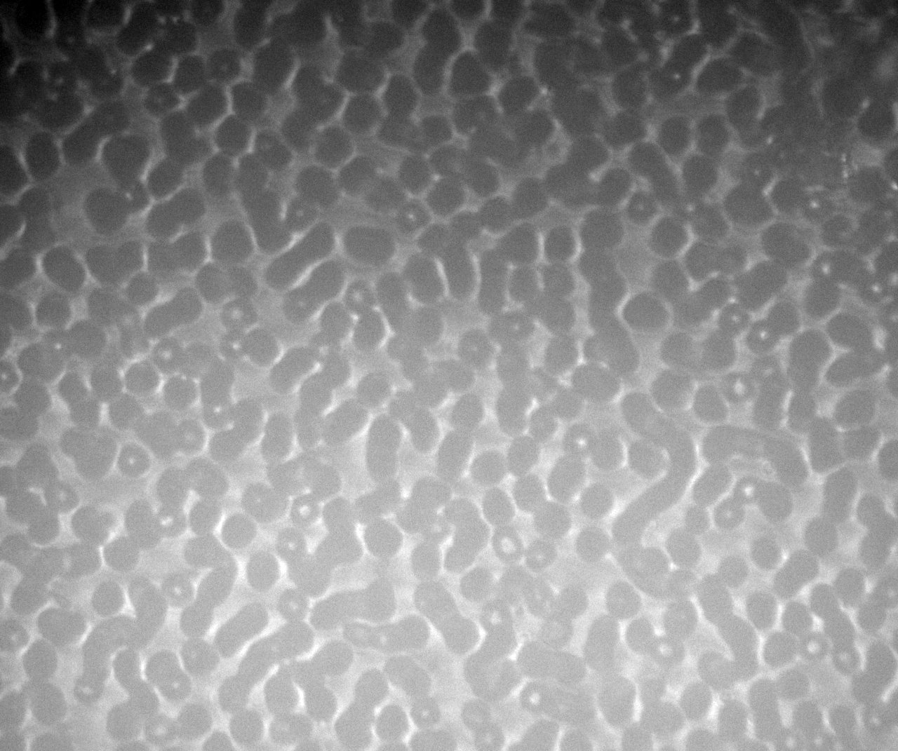
At the beginning, you will likely see an out-of-focus image like the one below.

Loosen the set screws of the camera. Carefully adjust the position of the camera along the cage rods until an in focus image is formed.

Depending on the lighting conditions, the image may not have good contrast. This does not matter. Just make the far away object in focus by finding the correct position of the camera.
Tighten the set screws once the image is in focus.
11
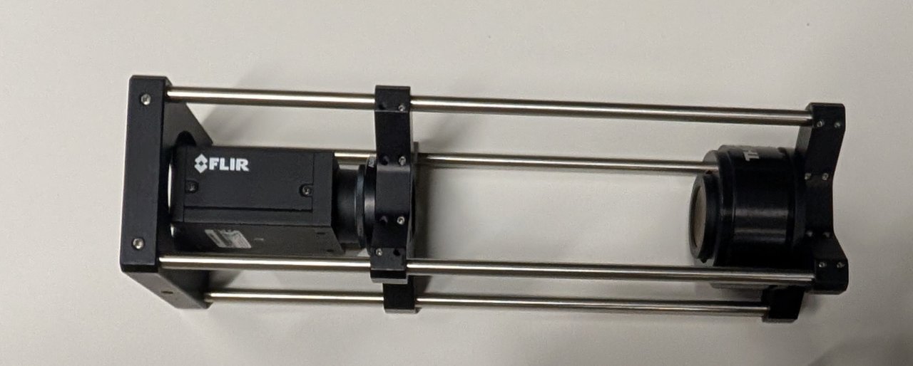
Attach the cage plate to the end of the cage rods. This will be used to mount the camera/tube lens assembly to the optical table in a later chapter.
You should now have a fully assembled, fixed focal length camera system.
Set up Micro-Manager
Micro-Manager is open source software for microscope control and automation. It allows you to control and coordinate many types of hardware from different vendors, often with little-to-no additional work.
As an ImageJ plugin, it also gives you image analysis capabilities on data as it is acquired far beyond what any camera manufacturer’s software allows.
We use Micro-Manager on several of our laboratory instruments. A basic understanding of how to use Micro-Manager is therefore essential to successful operation of these microscopes.
Download and Install the Latest Nightly Version
Micro-Manager comes in both stable and so-called “nightly” versions1. You will want to use the latest nightly version because it contains all the latest features and bug fixes.
Navigate to https://micro-manager.org/ and select the hamburger menu, then Downloads > Nightly Builds. Select Version 2.0 (Windows) and click the link to the most recent executable file, which should be at the top of the list.
Once the file is downloaded, run the installer and select all the default options.
Run Micro-Manager
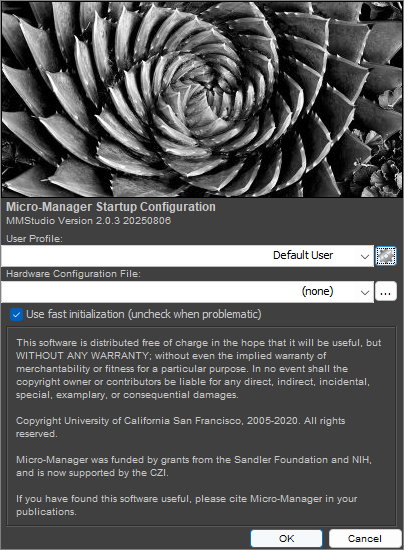
Launch Micro-Manager. Its startup screen will look something like the following:
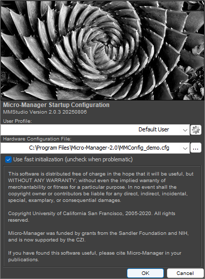
Select the MMConfig_demo configuration and select OK. You will have two windows open: the first is the ImageJ control panel. The second is the Micro-Manager control panel, as shown below:
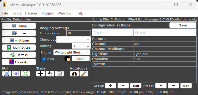
When you click the Live button, you should see a live image stream from the demo camera, which simulates a real camera by displaying a moving sine wave. You will alse see the image inspector window, which provides realtime information on the image’s histogram, bit depth, and other information.
Play with some of the settings in this window to get a feel for what you can do.
Micro-Manager Concepts
In order to use Micro-Manager at a basic level, it is important to understand the following concepts.
Device
A device is any piece of hardware that Micro-Manager controls. It could be a light source, a camera, a microscope stage, a filter wheel, a shutter, etc.
Device Properties
A device is akin to a state machine. The set of all its properties and their values make up the device’s state.
For example, a camera might have an exposure time property and a bit-depth property. A laser might have an output power property.
Some properties may be changed by the user, whereas others are read only. An example of a read only property would be a temperature sensor.
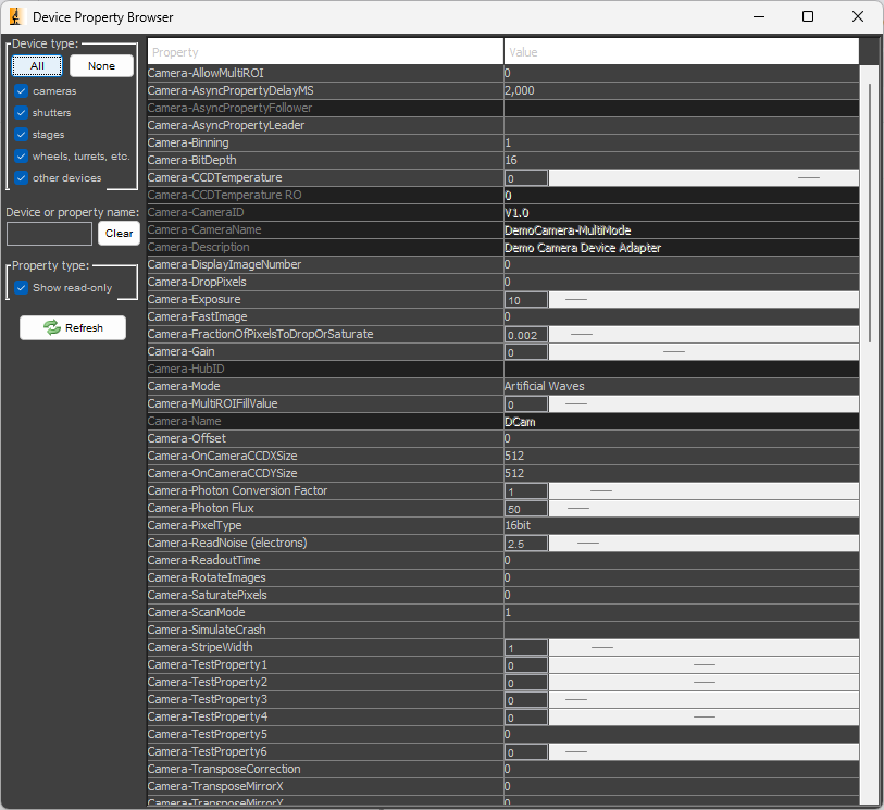
To see a list of all the device properties for all the currently configured devices, navigate to Devices > Device Property Browser.... You may also modify properties in this window.
The device property browser for the MMDemo configuration is shown below.
Device Adapter
Device adapters are what make Micro-Manager so powerful. A device adapter is a plugin for a device that allows it to work with Micro-Manager.
A device adapter must exist for a device to be used with Micro-Manager. If one does not exist, you can write one using the C++ programming language to make it work with Micro-Manager. Writing device adapters is outside the scope of this basic training course, however.
You may find a partial list of supported devices at the Micro-Manager website.
Configuration
The configuration is the set of all devices to be controlled by Micro-Manager, as well as additional settings like desired default values.
Configurations allow you to select hardware and settings for different experiments.
In the following section, we will configure Micro-Manager to control the Flir camera for our microscope.
Create a New Configuration
0
Close Micro-Manager if it is already open.
Connect the camera to your PC and launch Micro-Manager. Select (none) for the Hardware Configuration File and click Ok.
1
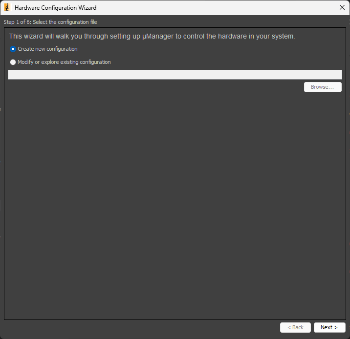
In the Micro-Manager control panel, navigate to Devices > Hardware Configuration Wizard.... Select Create new configuration and click Next >.
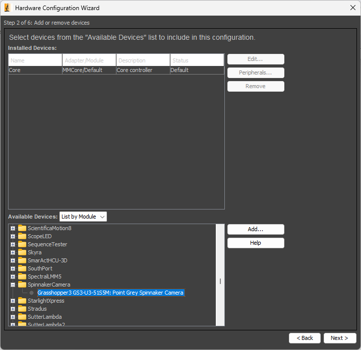
2
In the next window, scroll down the list of available devices until you find the device called SpinnakerCamera. Expand the item to find our Grasshopper camera. Select it, and click Add... and then OK. ClickNext > through the remaining windows. At the end, save the configuration file somewhere that makes sense.
Troubleshooting
Can’t see a device called SpinnakerCamera? The Grasshopper camera does not appear in the list? Do you receive an error immediately after creating the configuration? Try the following things to troubleshoot.
- Restart Micro-Manager. Devices need to be plugged in before Micro-Manager starts for them to be recognized.
- Ensure that you installed the correct version of the Spinnaker SDK during the camera setup.
- Be sure that the camera is recognized by SpinView. In general, if a device can’t be used by its manufacturer’s software, then it will not work in Micro-Manager.
3
Once back at the Micro-Manager control panel, click the Live button. You should see a live image stream in the preview window and the image inspector showing a histogram of the pixel values.
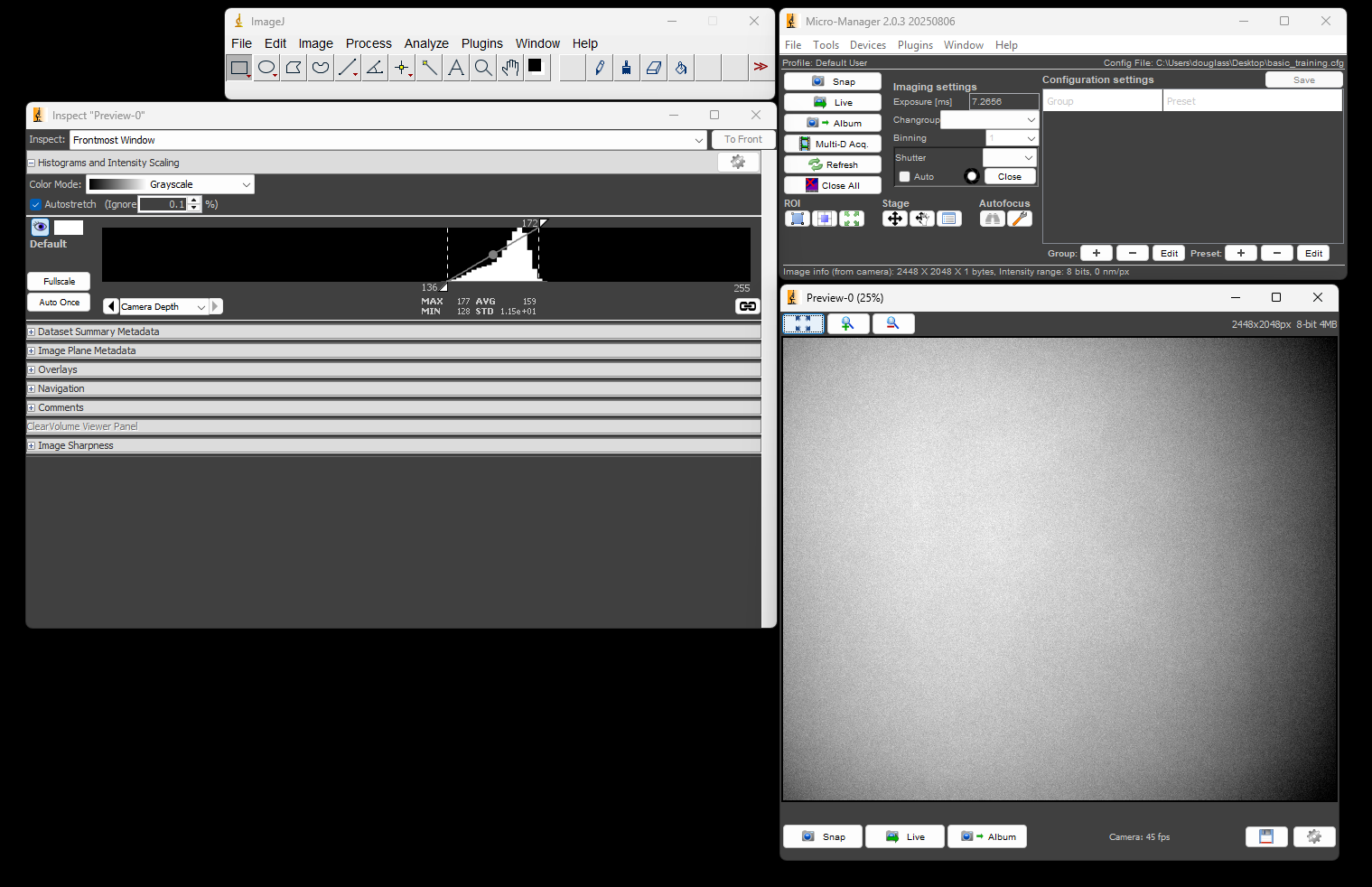
At this point you have configured Micro-Manager to control the camera. Feel free to play with settings such as the exposure time, or go into the Device Property Browser to see what camera properties can be modified.
-
A new nightly version is created at the end of any day where the source code changes. It’s called “nightly” because it used to be built once a day, regardless of whether the source code changed. ↩
Discussion
Infinity Corrected Optics
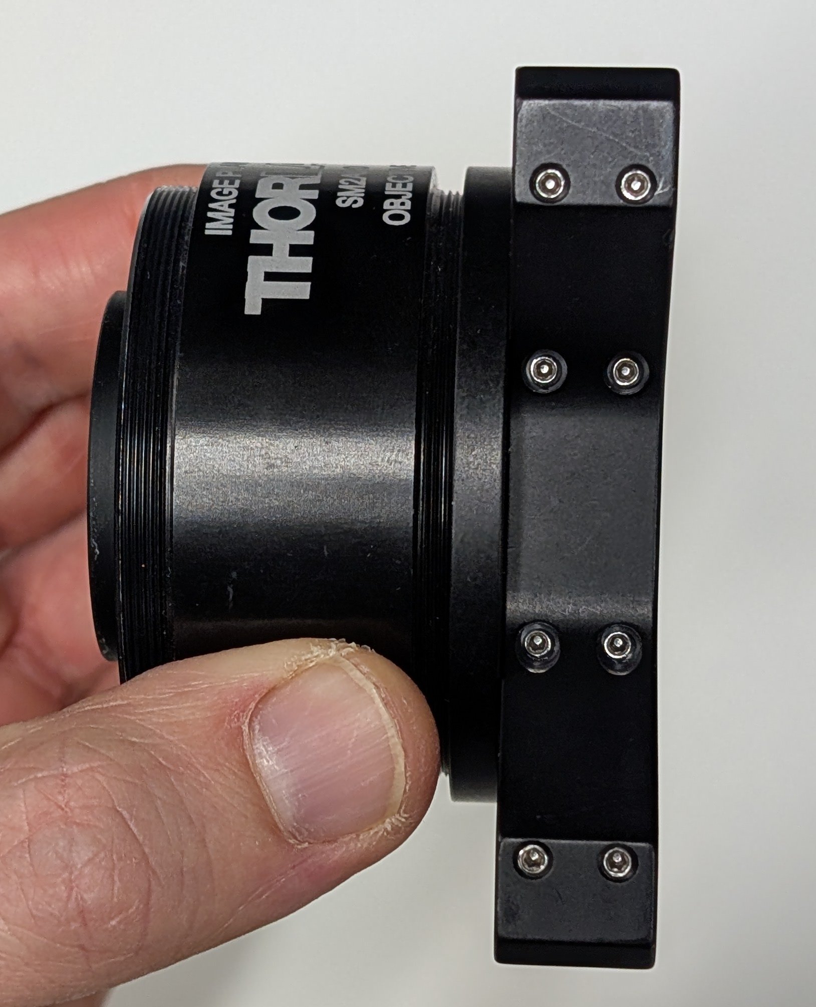
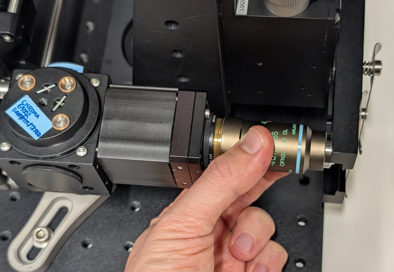
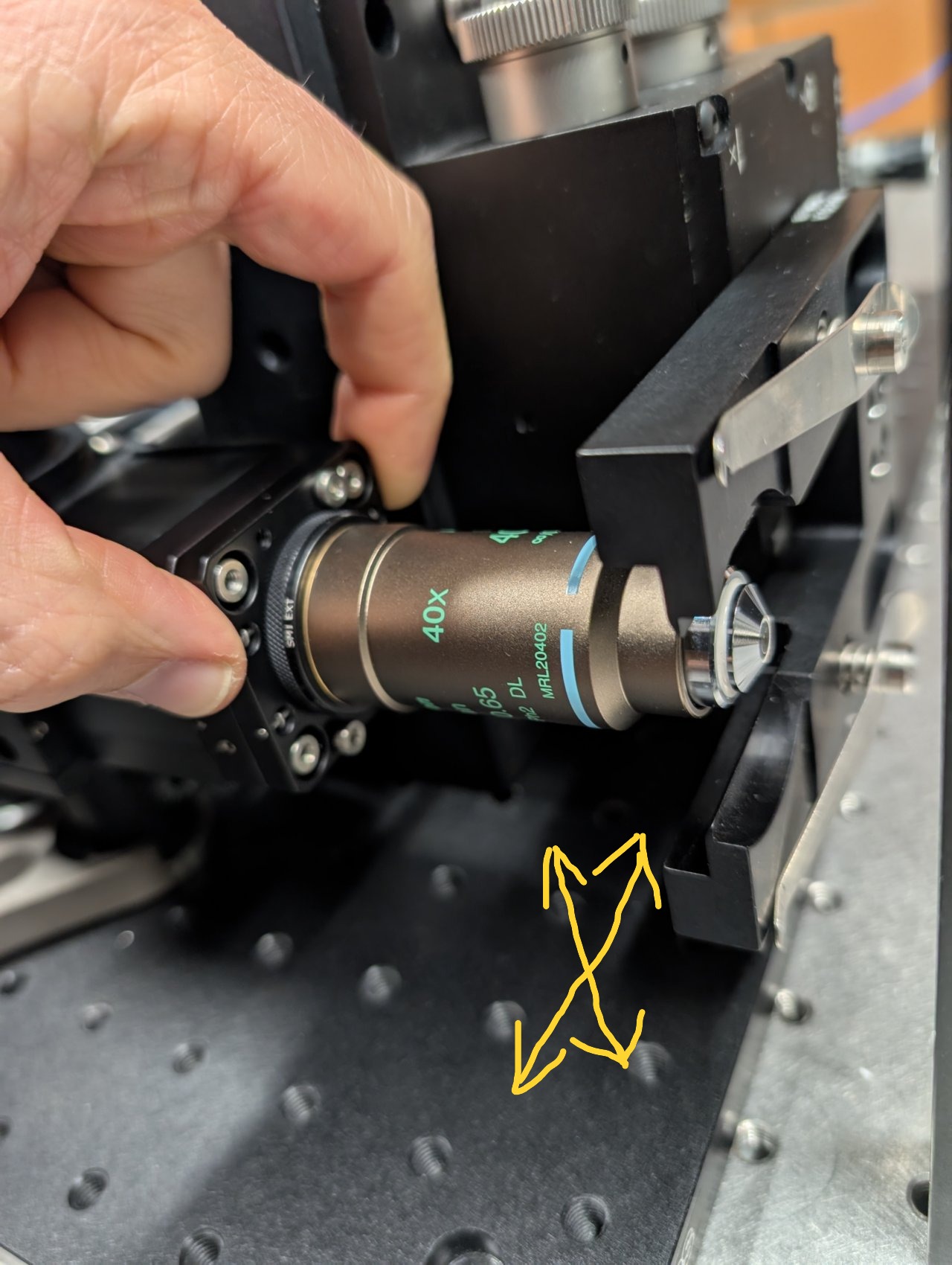
Nearly all microscopes that you will encounter within our research lab use infinity corrected optics, so it is important to understand what this means.
An infinity corrected objective will have an infinity symbol on the barrel like the one in the photo below.
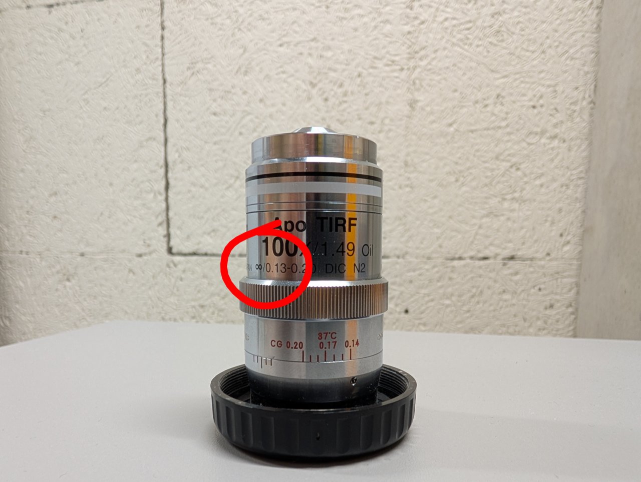
By design, the sample is located at the front focal plane of an infinity corrected objective. This means that the image of the sample is formed an infinite distance away from the objective on the other side. An image at infinity cannot be seen with a camera1, so we require a second a lens to form a real image in the camera plane. This second lens is known as the tube lens.
But why is the image of the sample formed at infinity in the first place? Recall the thin lens formula from your introductory physics class:
\[ \frac{1}{s} + \frac{1}{s’} = \frac{1}{f} \]
Here, \( s \) is the distance from the lens to the object, \( s’ \) is the distance from the lens to the image, and \( f \) is the focal length of the lens. If the object distance is equal to the focal length, then \( s = f \). But then we have
\[ \frac{1}{s’} = 0 \]
The only way to satisfy this equation is by requiring that the image distance be infinitely large. This is what we mean when we say that the image is “at infinity.”
The situation is illustrated below. An object lies at a distance \( s = f \) from a thin lens with a positive focal length, which is drawn as a vertical line with arrows at each end. Rays from a single object point emerge from the lens parallel to one another. The image plane is defined as the plane where the rays intersect one another. But the rays are parallel, so they intersect at infinity.

The Camera Sensor is in the Focal Plane of the Tube Lens
By the same logic, the camera sensor must be in the focal plane of the tube lens of a properly aligned, infinity corrected system. The image at infinity created by the objective serves as the object for the tube lens so that we have
\[ \frac{1}{\infty} + \frac{1}{s’} = \frac{1}{f} \]
or \( s’ = f \).
This situation is illustrated below. Parallel rays representing an object at infinity are brought to a focus in the focal plane of a thin lens.

Focusing on a Distant Object Aligned the Camera Sensor with the Tube Lens Focal Plane
When we looked at far away clouds or mountains using our fixed focal length camera, we essentially were looking at objects at infinity. By adjusting the separation between the camera and tube lens such that a clear image was formed, we were placing the camera sensor in the focal plane of the tube lens.
Why Can’t I Just Use a Ruler?
The tube lens has a 200 mm focal length. Many students are tempted to use a ruler to separate the camera from the tube lens by 200 mm, but this is not the correct way to put the camera sensor in the focal plane of the tube lens for two reasons.
- The camera sensor sits inside the camera housing at a distance of about 17 mm from the opening, so any distance measurement must account for this.
- Focal lengths are measured relative to imaginary planes called the principal planes of a lens. The locations of these planes depend on the details of the lens, i.e. glass surface curvatures, refractive indexes, number of components, etc. We cannot look at any given lens and say with certainty where the principal planes are located without performing calculations.
So if we don’t know where the principal planes are, then we don’t know the point from where we need to measure to find the focal plane.
The advantage to modeling a system with the principal planes is that we can abstract over all the details of a real lens and replace them with just two planes.
The Space between the Objective and Tube Lens is called Infinity Space
In the schematic below, \( O / O’ \) and \( T / T’ \) are the principal planes for the microscope objective and tube lens, respectively. \( f_{obj} \) and \( f_{TL} \) denote the focal lengths of the objective and tube lens, respectively. Light rays from an off-axis object point are collected by the objective and made parallel after the objective’s second prinicpal plane. The same rays are refocused by the tube lens onto the camera sensor.

The space between the objective and tube lens is called the infinity space because the image of the sample is located at infinity within this space.
Prior to the development of infinity corrected systems, microscope objectives formed their images at a fixed distance from the objective, called the tube length. By convention, this distance was usually around 160 mm. A second lens, the eye piece would send this intermediate image to infinity so that it could be viewed by the eye. Modern microscopy requires that additonal optical elements be placed after the objective, such as dichroic mirrors and filters. Upon insertion into the optical path, these additonal elements displace the location of the image formed by a traditional objective due the refractive index difference between the element’s material and air. This in turn forces the microscopist to refocus the image as elements are inserted and removed. It also results in a slightly different magnification for different elements.
Infinity corrected systems do not suffer from these problems because the intermediate image is located at infinity. As a result, the final image will not change the position when additonal elements are inserted into the infinity space between the objective and tube lens.
Think in Terms of Conjugate Planes
Consider the planes denoted by the dashed lines in the above figure. These denote the sample plane and its image. Rays from one point in one of these planes are mapped to a single point in another.
Any pair of planes that satisfies this mapping are called conjugate planes. Another set of important conjugate planes corresponds to the back focal plane (BFP) of the objective and its images. Schematics of microscopes can almost always be understood by asking where the conjugates are for the sample and objective BFP are.
The Thin Lens Equation is Compatible with the Principal Planes
Can we really use the thin lens equation if we are dealing with thick lenses represented as principal planes?
In short, yes. While a complete discussion about this goes beyond the scope of this basic training course, one can show that the ray transfer matrix of a thick lens is identical to a thin lens so long as the object space and image space coordinate systems are chosen with respect to origin in the points where the object space and image space prinicpal planes intersect the optical axis, respectively.
For more information, see section 2.5.7 here.
-
An image at infinity can be seen by eye, however. Do you know why? ↩
Questions
-
What is the difference between an excitation filter and a dichroic mirror?
-
Why do we use an emission filter in addition to a dichroic mirror in the fluorescence light path?
-
True or false: fluorescence light has a shorter wavelength than that of the excitation light.
-
What are the differences between industrial CMOS and scientific CMOS (sCMOS) cameras?
-
True or false: A camera with an exposure time of 20 ms necessarily acquires frames at a rate of 50 frames per second.
-
Does the distance between the objective and the tube lens matter? Why or why not?
-
Why do we do fluorescence imaging with epi-illumination and not transillumination?
Alignment
In this chapter we will finish the construction of our fluoresence microscope in two parts. In the first, we will finish the fluoresence light path, also known as the emission path.
In the second part, we will build and align the optics for the excitation light path.
Construct the Microscope Emission Path
Parts List
Below is the parts list for this section of the basic training course. Note that some of the parts used in the course are now obsolete. In these cases the parts listed below are the closest current match to the obsolete parts.
| Part | Manf. Part No. | Quantity | URL |
|---|---|---|---|
| Chroma 69002 ET - DAPI/FITC/Texas Red® Filter Set | 69002 | 1 | https://www.chroma.com/products/sets/69002-et-dapi-fitc-texas-red |
| Nikon CFI Plan Achro DL40x Microscope Objective | MRL20402 | 1 | https://www.microscope.healthcare.nikon.com/products/optics/selector/comparison/-1703 |
| 3-Axis NanoMax Stage, Differential Drives, Closed-Loop Piezos, Metric | MAX311D/M | 1 | https://www.thorlabs.com/thorproduct.cfm?partnumber=MAX311D/M |
| Microscopy Slide Holder | MAX3SLH | 1 | https://www.thorlabs.com/thorproduct.cfm?partnumber=MAX3SLH |
| Ø1“ Broadband Dielectric Mirror, 400 - 750 nm | BB1-E02 | 1 | https://www.thorlabs.com/thorproduct.cfm?partnumber=BB1-E02 |
| Right-Angle Kinematic Mirror Mount with Tapped Cage Rod Holes, 30 mm Cage System and SM1 Compatible, M4 and M6 Mounting Holes | KCB1/M | 1 | https://www.thorlabs.com/thorproduct.cfm?partnumber=KCB1/M |
| 30 mm Cage Cube, Ø6 mm Through Holes | C6WR | 1 | https://www.thorlabs.com/thorproduct.cfm?partnumber=C6WR |
| 30-mm-Cage-Compatible Rectangular Filter Mount | FFM1 | 1 | https://www.thorlabs.com/thorproduct.cfm?partnumber=FFM1 |
| Kinematic Cage Cube Platform for C4W/C6WR, Metric | B4C/M | 1 | https://www.thorlabs.com/thorproduct.cfm?partnumber=B4C/M |
| Coarse ±1 mm XY Slip Plate Positioner, 30 mm Cage Compatible, Metric | SPT1C/M | 1 | https://www.thorlabs.com/thorproduct.cfm?partnumber=SPT1C/M |
| Externally SM1-Threaded End Cap | SM1CP2 | 1 | https://www.thorlabs.com/thorproduct.cfm?partnumber=SM1CP2 |
| Rod Adapter for Ø6 mm ER Rods, L = 0.27“ | ERSCB | 4 | https://www.thorlabs.com/thorproduct.cfm?partnumber=ERSCB |
| Cage Assembly Rod, 1/4“ Long, Ø6 mm | ER025 | 4 | https://www.thorlabs.com/thorproduct.cfm?partnumber=ER025 |
| Cage Assembly Rod, 1“ Long, Ø6 mm | ER1 | 4 | https://www.thorlabs.com/thorproduct.cfm?partnumber=ER1 |
| Cage Assembly Rod, 2“ Long, Ø6 mm | ER2 | 4 | https://www.thorlabs.com/thorproduct.cfm?partnumber=ER2 |
| Ø12.7 mm Optical Post, SS, M4 Setscrew, M6 Tap, L = 20 mm | TR20/M | 1 | https://www.thorlabs.com/thorproduct.cfm?partnumber=TR20/M |
| Ø12.7 mm Optical Post, SS, M4 Setscrew, M6 Tap, L = 30 mm | TR30/M | 2 | https://www.thorlabs.com/thorproduct.cfm?partnumber=TR30/M |
| Ø12.7 mm Post Holder, Spring-Loaded Hex-Locking Thumbscrew, L=20 mm | PH20/M | 1 | https://www.thorlabs.com/thorproduct.cfm?partnumber=PH20/M |
| Ø12.7 mm Post Holder, Spring-Loaded Hex-Locking Thumbscrew, L=30 mm | PH30/M | 1 | https://www.thorlabs.com/thorproduct.cfm?partnumber=PH30/M |
| Clamping Fork for Ø1.25“ Pedestal Bases, 44.4 mm Counterbored Slot, M6 x 1.0 Captive Screw | CF175C/M | 3 | https://www.thorlabs.com/thorproduct.cfm?partnumber=CF175C/M |
| Ø31.8 mm Studded Pedestal Base Adapter, M6 Threads | BE1/M | 3 | https://www.thorlabs.com/thorproduct.cfm?partnumber=BE1/M |
| Adapter with External SM1 Threads and Internal M25 x 0.75 Threads | SM1A12 | 1 | https://www.thorlabs.com/thorproduct.cfm?partnumber=SM1A12 |
| 30 mm Cage System Cover, 24“ Long, Pack of 4 | C30L24 | 1 | https://www.thorlabs.com/thorproduct.cfm?partnumber=C30L24 |
| SM1 Lens Tube, 0.30“ Thread Depth, One Retaining Ring Included | SM1L03 | 2 | https://www.thorlabs.com/thorproduct.cfm?partnumber=SM1L03 |
| Aluminum Breadboard, 300 mm x 450 mm x 12.7 mm, M6 Taps | MB3045/M | 1 | https://www.thorlabs.com/thorproduct.cfm?partnumber=MB3045/M |
| Large Right-Angle Bracket, M6 Holes | AP90RL/M | 1 | https://www.thorlabs.com/thorproduct.cfm?partnumber=AP90RL/M |
| M6 x 1.0 Stainless Steel Cap Screw, 16 mm Long, 25 Pack | SH6MS16 | 6* | https://www.thorlabs.com/thorproduct.cfm?partnumber=SH6MS16 |
| 1/4“ Washer, M6 Compatible, Stainless Steel, 100 Pack | W25S050 | 6* | https://www.thorlabs.com/thorproduct.cfm?partnumber=W25S050 |
- Only a small quantity from larger pack is required.
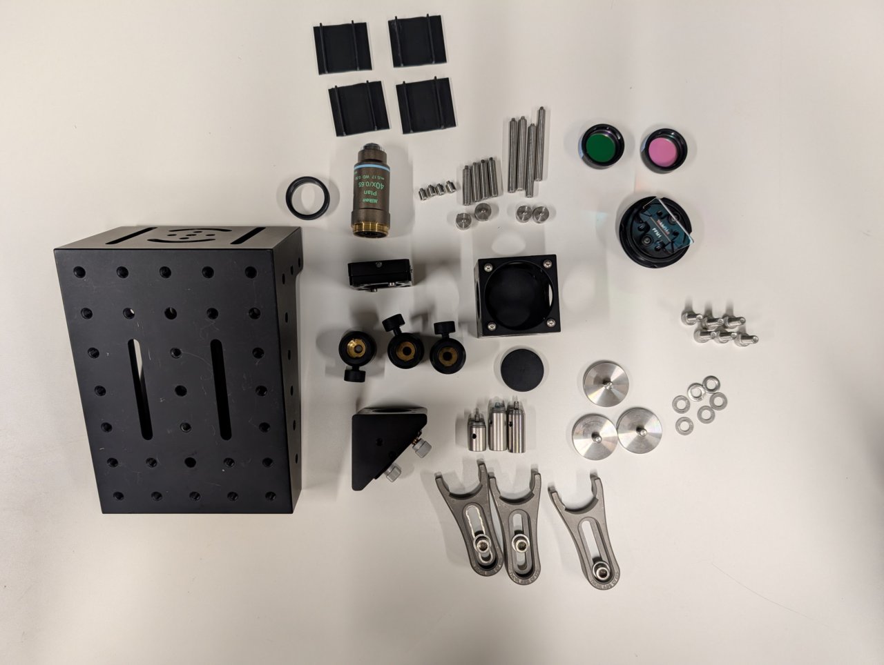
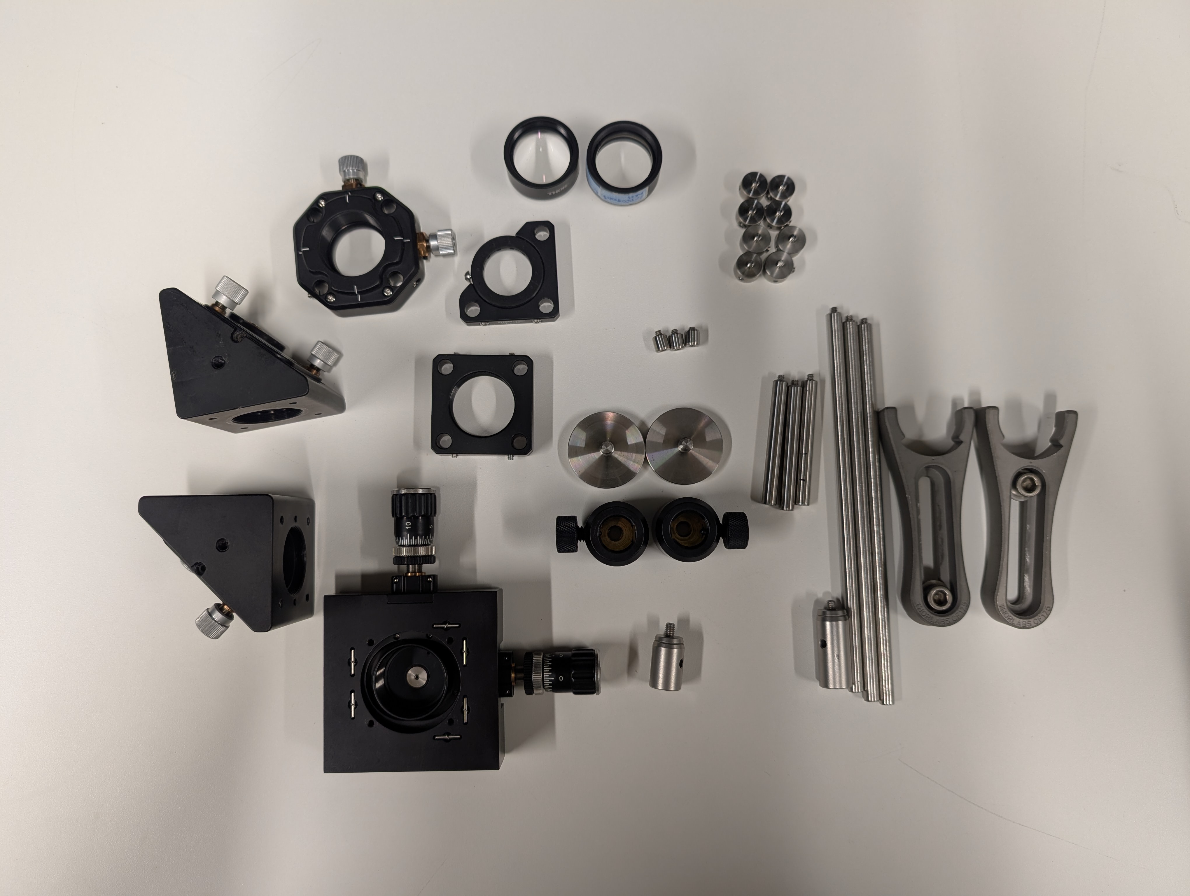
Not shown: 3-Axis NanoMax Stage and Microscopy Slide Holder
Instructions
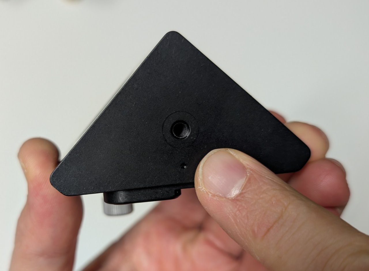
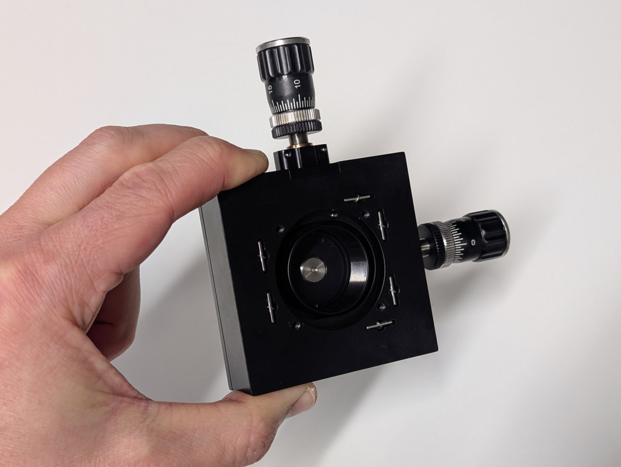
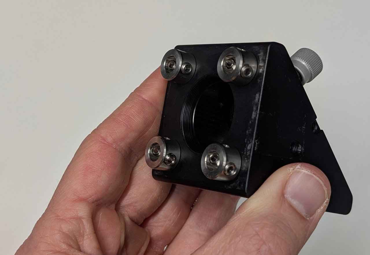
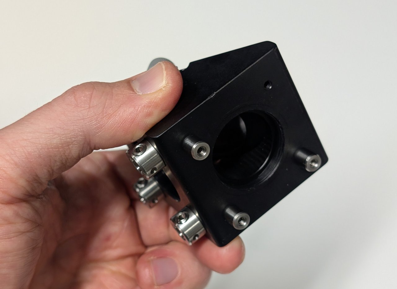
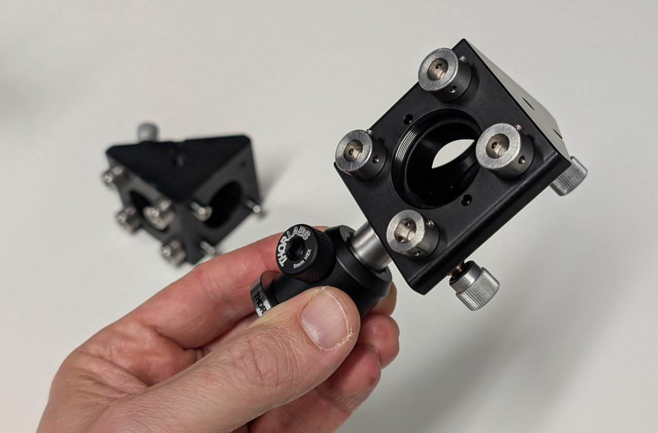
0
Find the side of the right-angle mirror mount with a dot on it. Take this side to be the bottom.
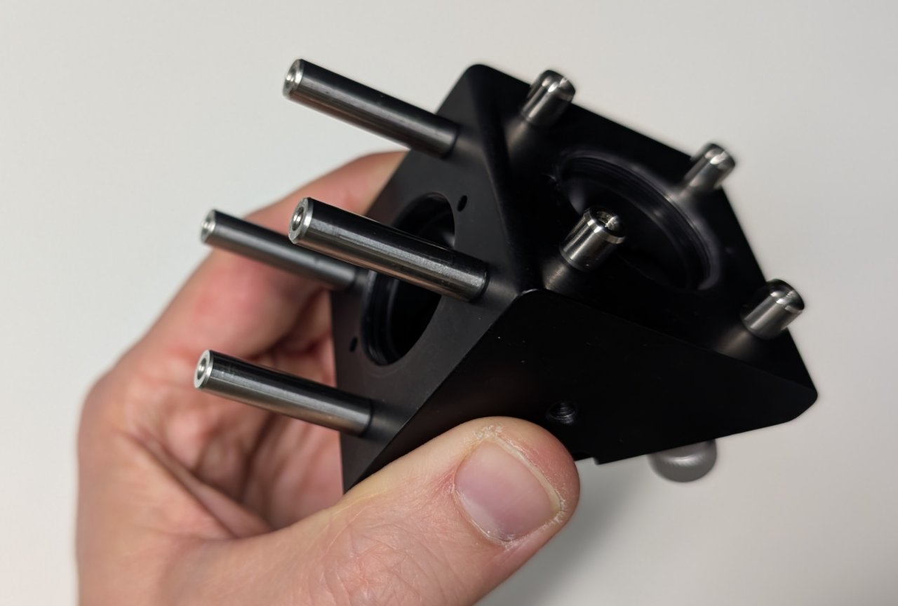
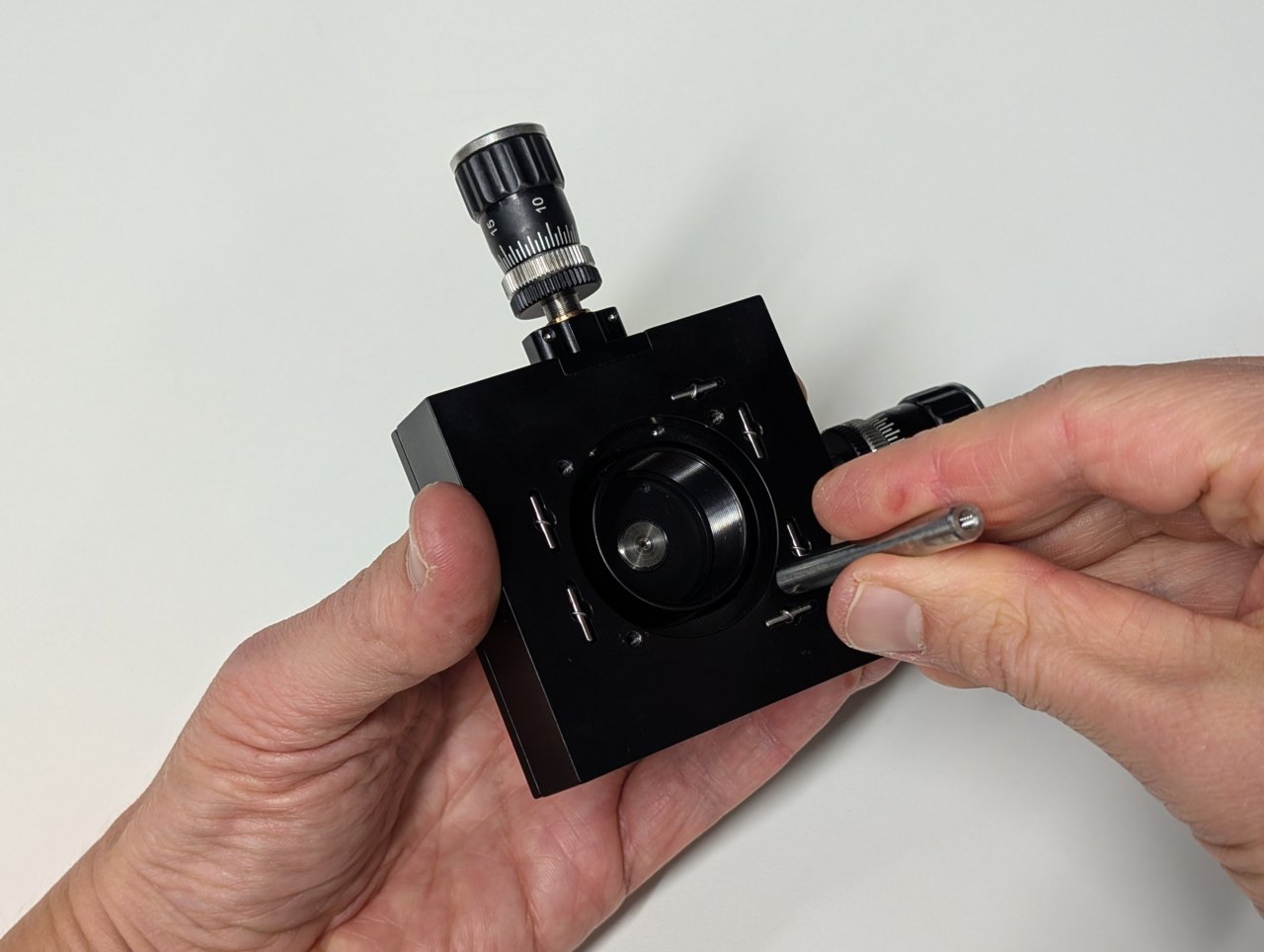
1
Attach 4, 0.25“ cage rods to the right-angle mirror mount as shown.
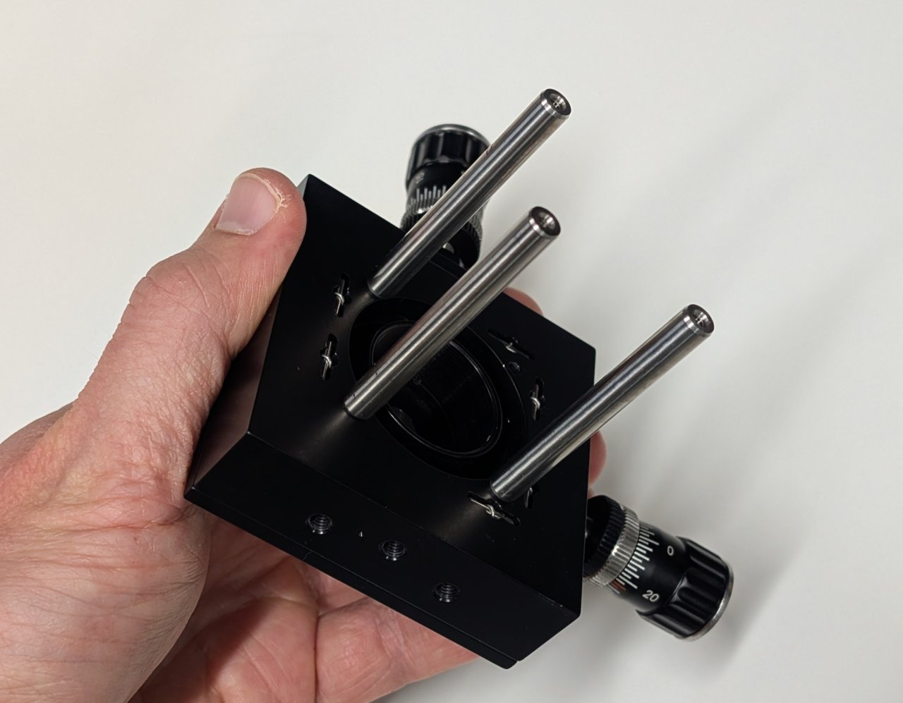
Attach 4, 1“ cage rods to the other side.
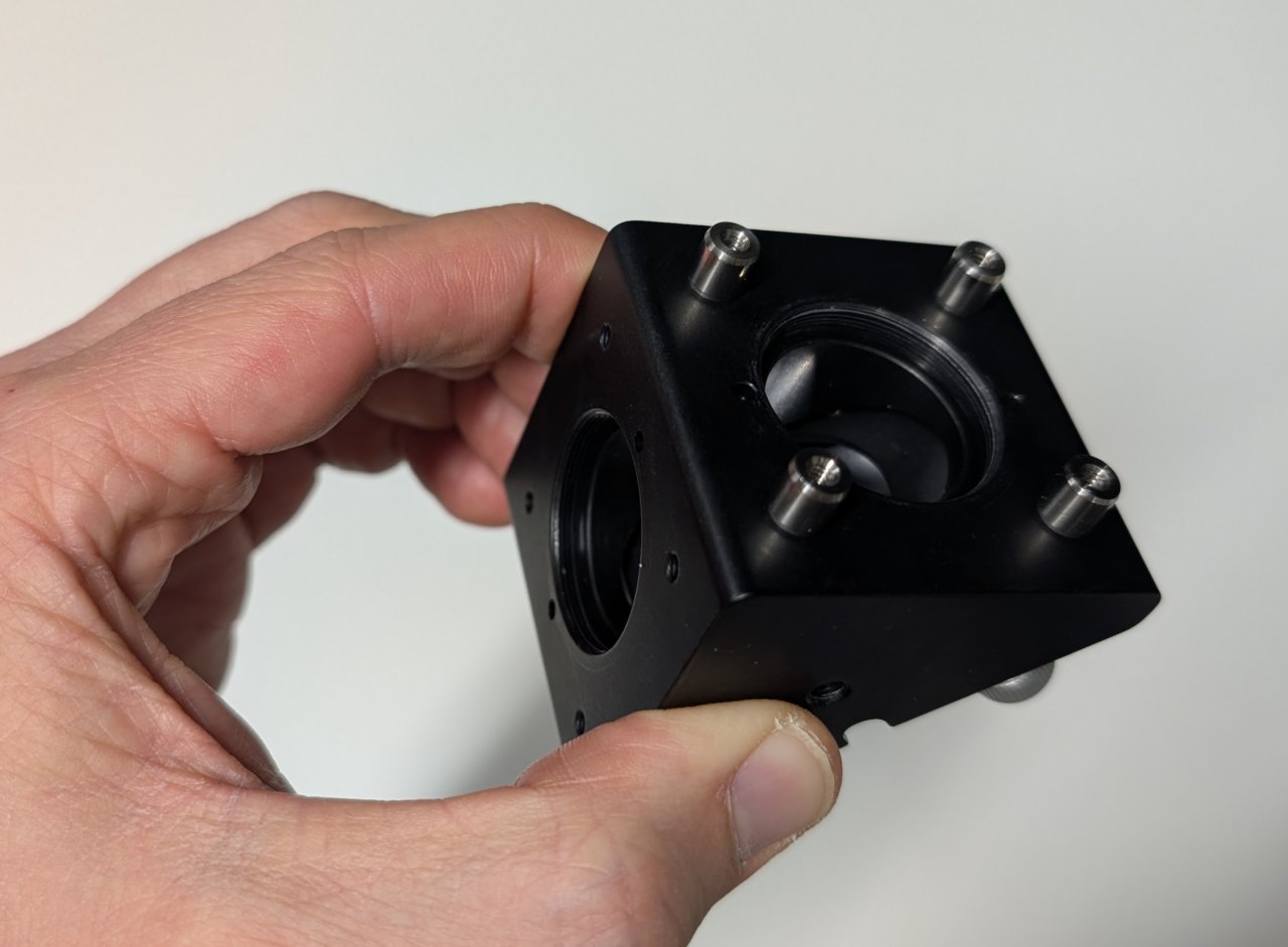
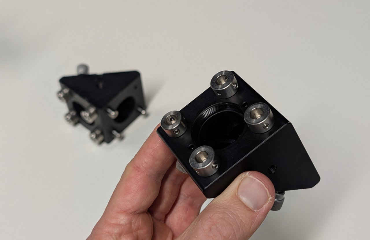
2
Attach 4 cage rod adapters to the exterior of the 30 mm cage cube as shown.
Screw the lens tube containing the emission filter into the SM1 threaded hole on the same side as the cage rod adapters.
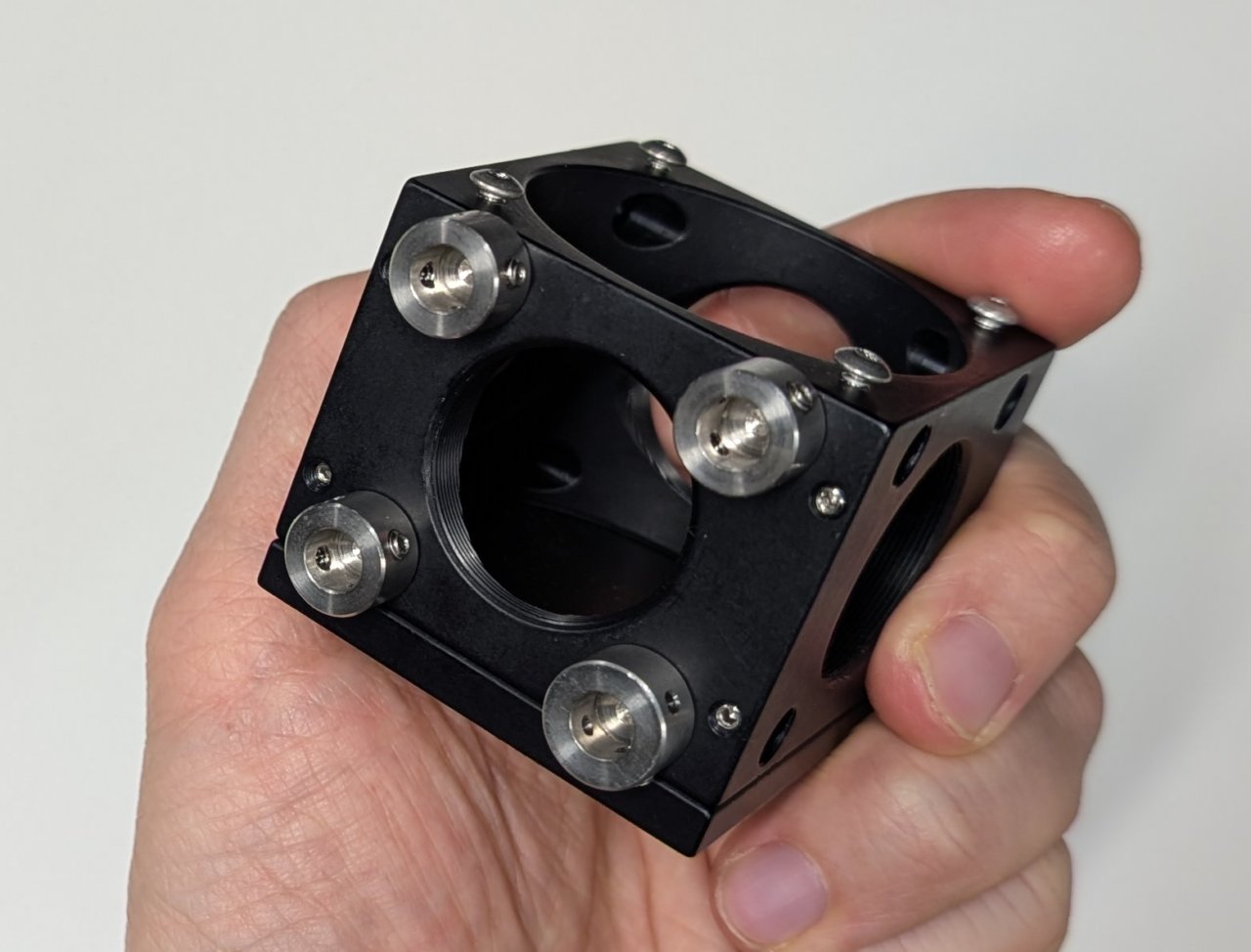
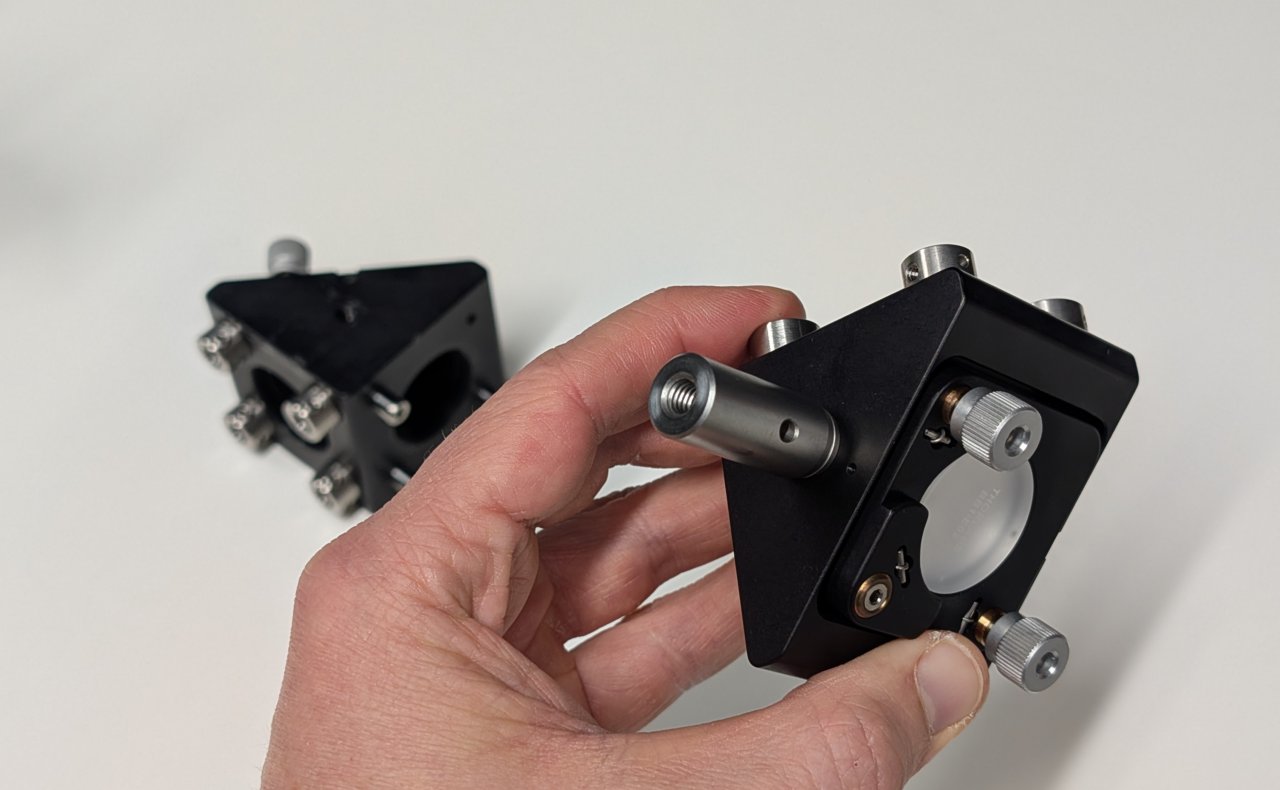
3
Attach the cage cube to the right-angle mirror mount using the 0.25“ cage rods and cage rod adapters. Remember to keep the side of the right-angle mirror mount with the dot facing down.
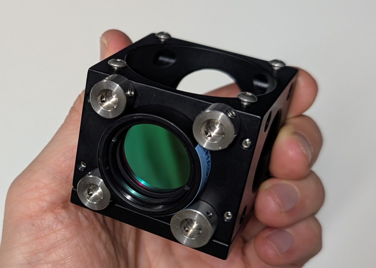
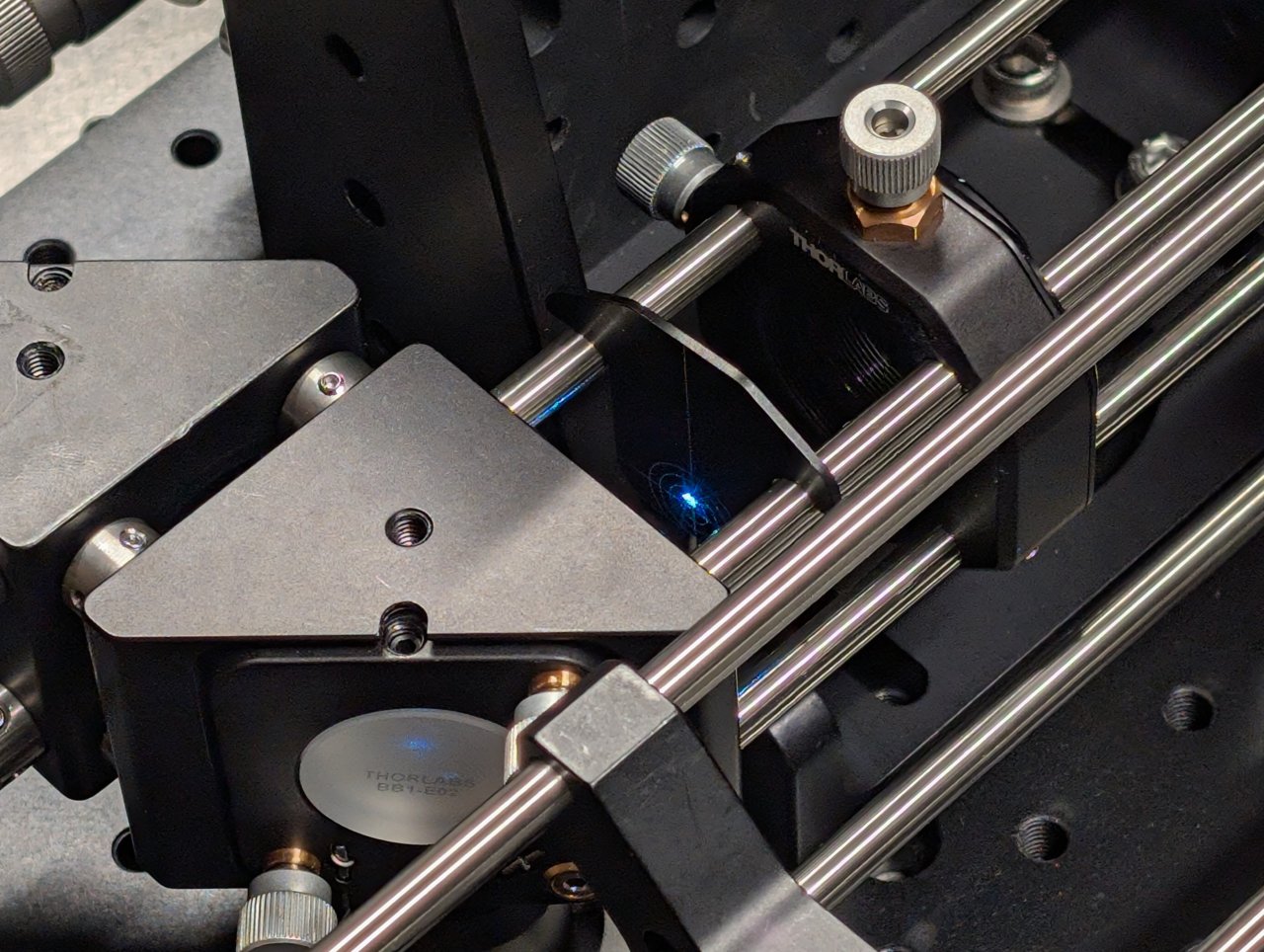
4
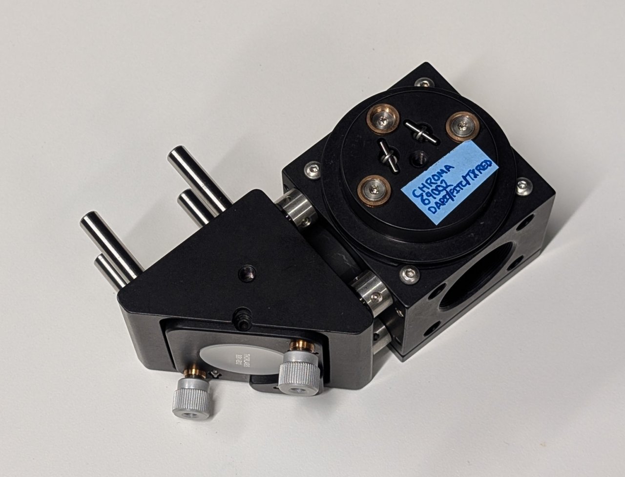
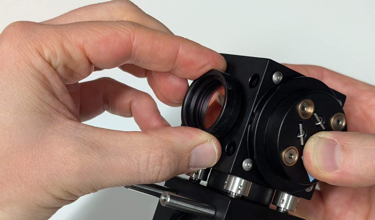
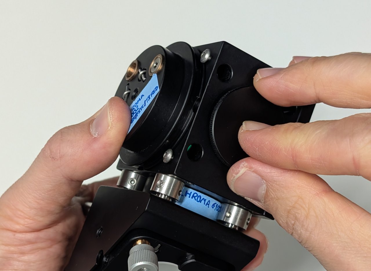
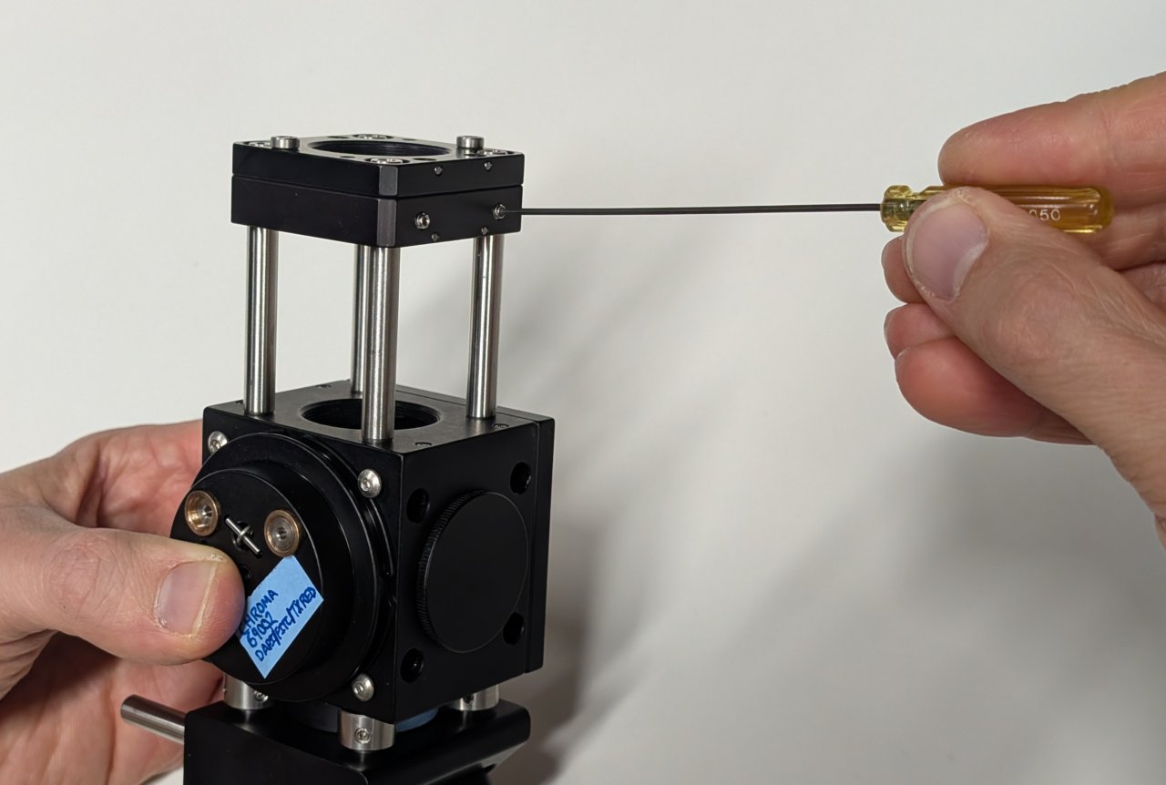
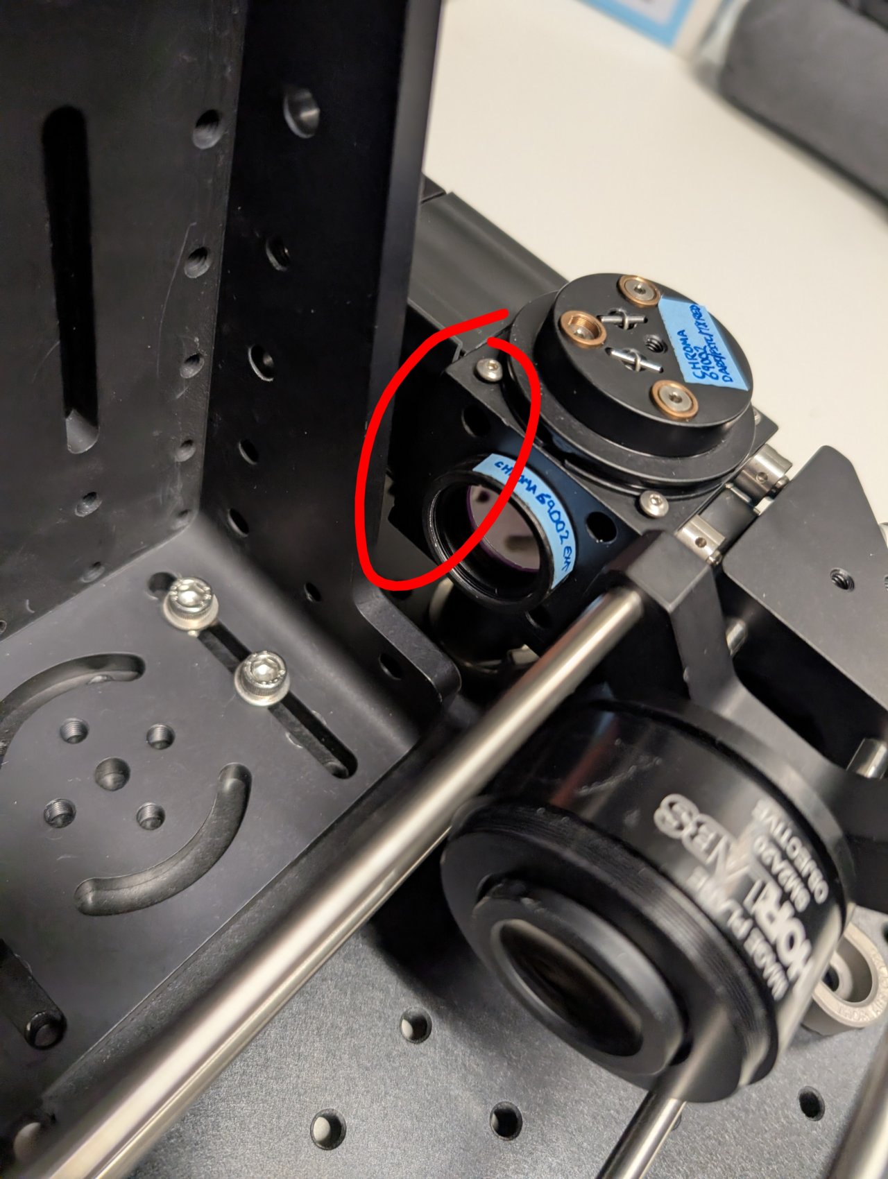
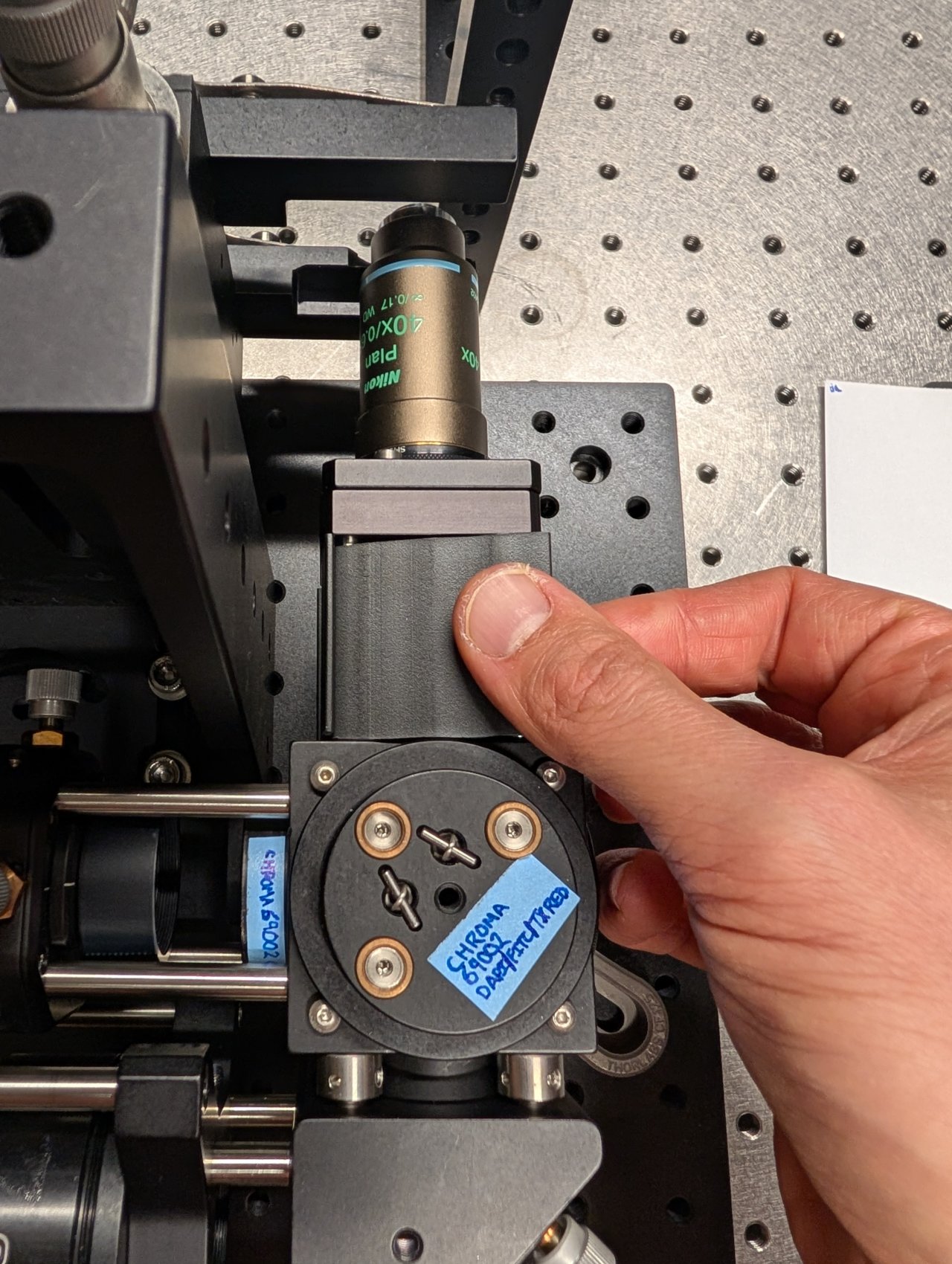
Note the arrow on the side of the dichroic mirror. This arrow points to the side with the dielectric coating and should face towards the sample.
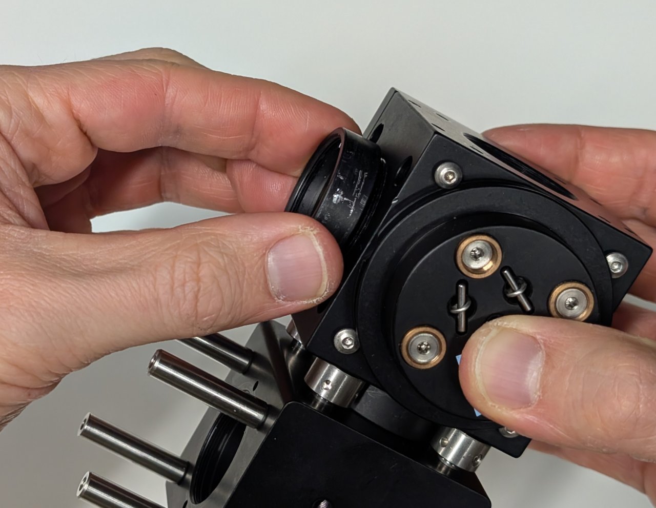
Insert the filter and its kinematic platform into the cage cube.
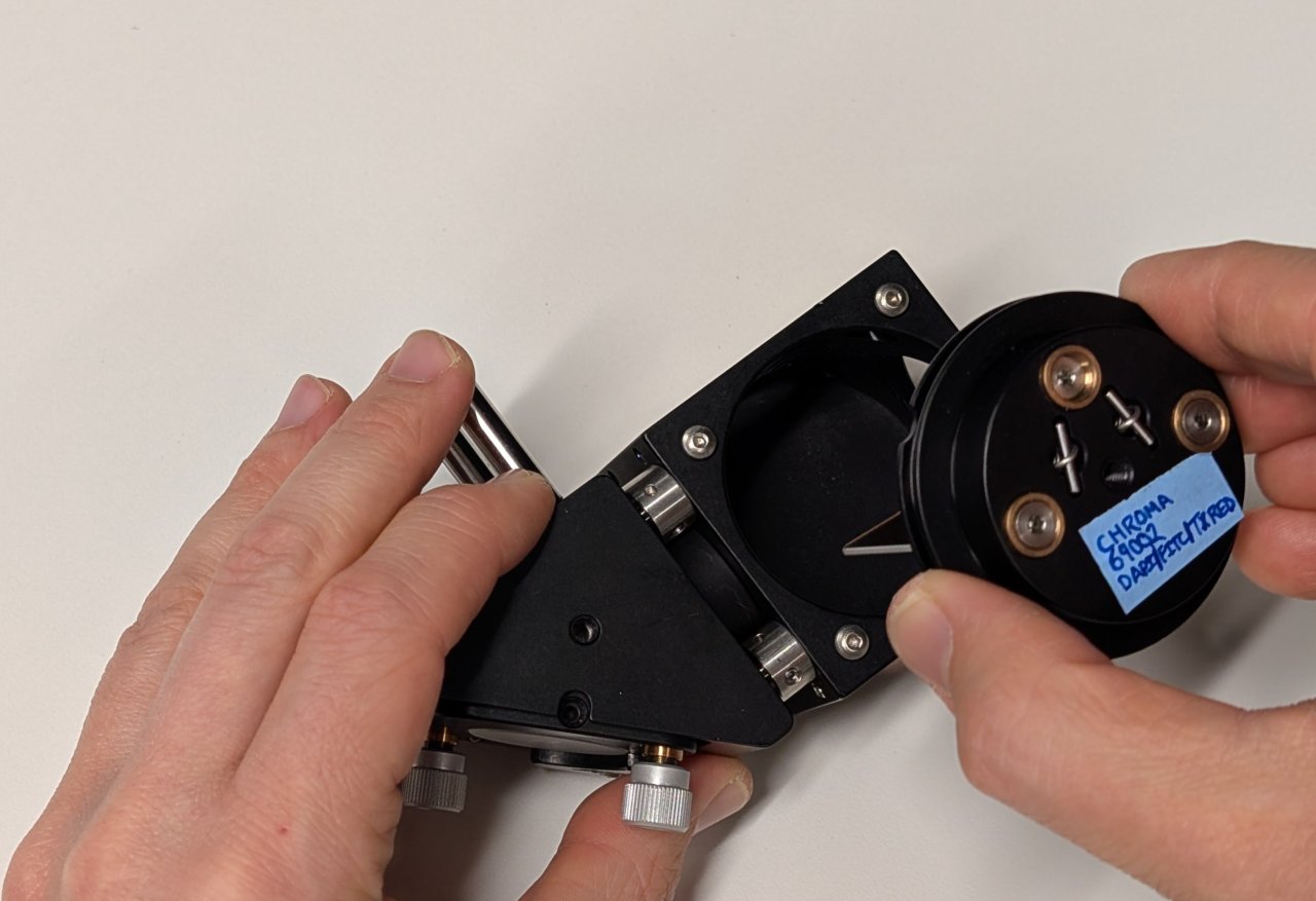
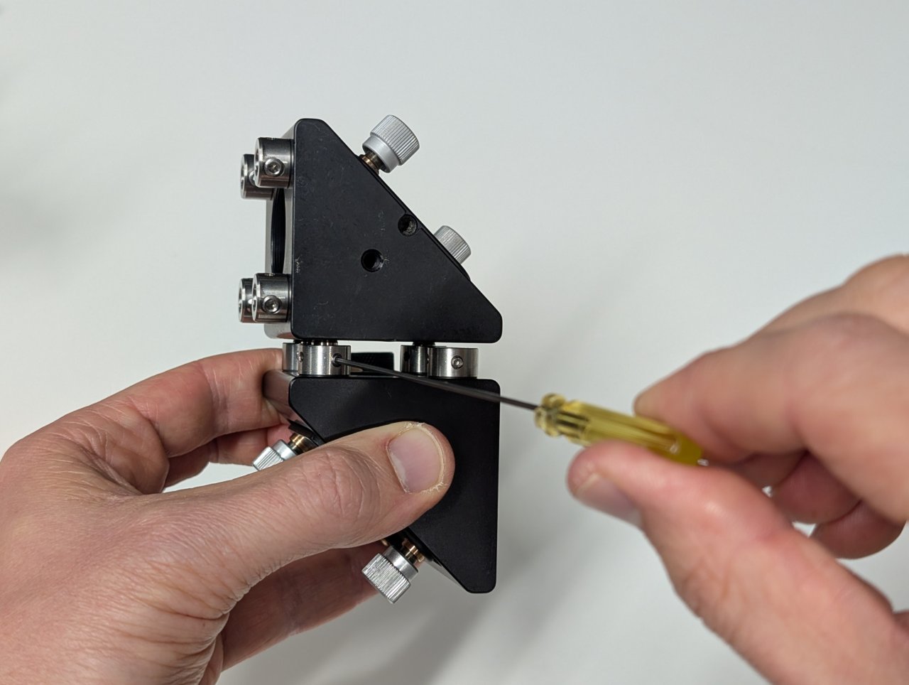
5
Rotate the platform by approximately 45 degrees, ensuring that the side of the dichroic mirror with the coating faces away from the mirror.
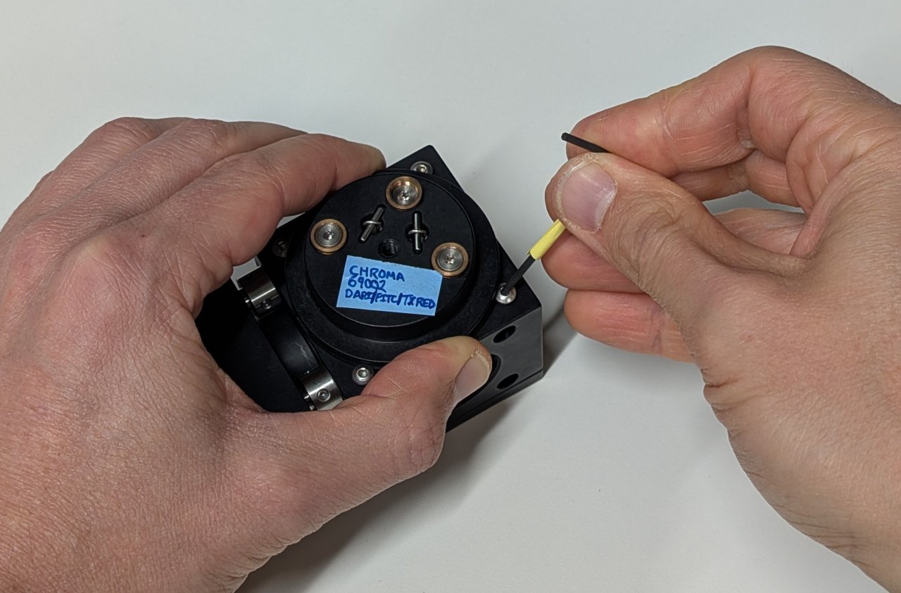
Tighten the screws on the cage cube. (They are imperial in the image shown!)
###6
Screw the lens tube containing the excitation filter into the cage cube.
7
Screw the SM1-threaded end cap into the hole on the cage cube that is opposite the excitation filter.
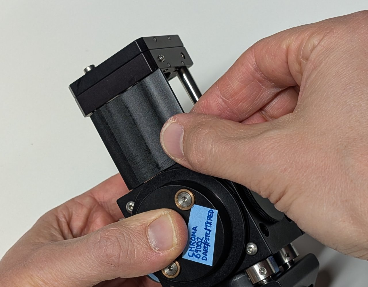
8
Attach 4, 2“ long cage rods to the top of the cage cube.
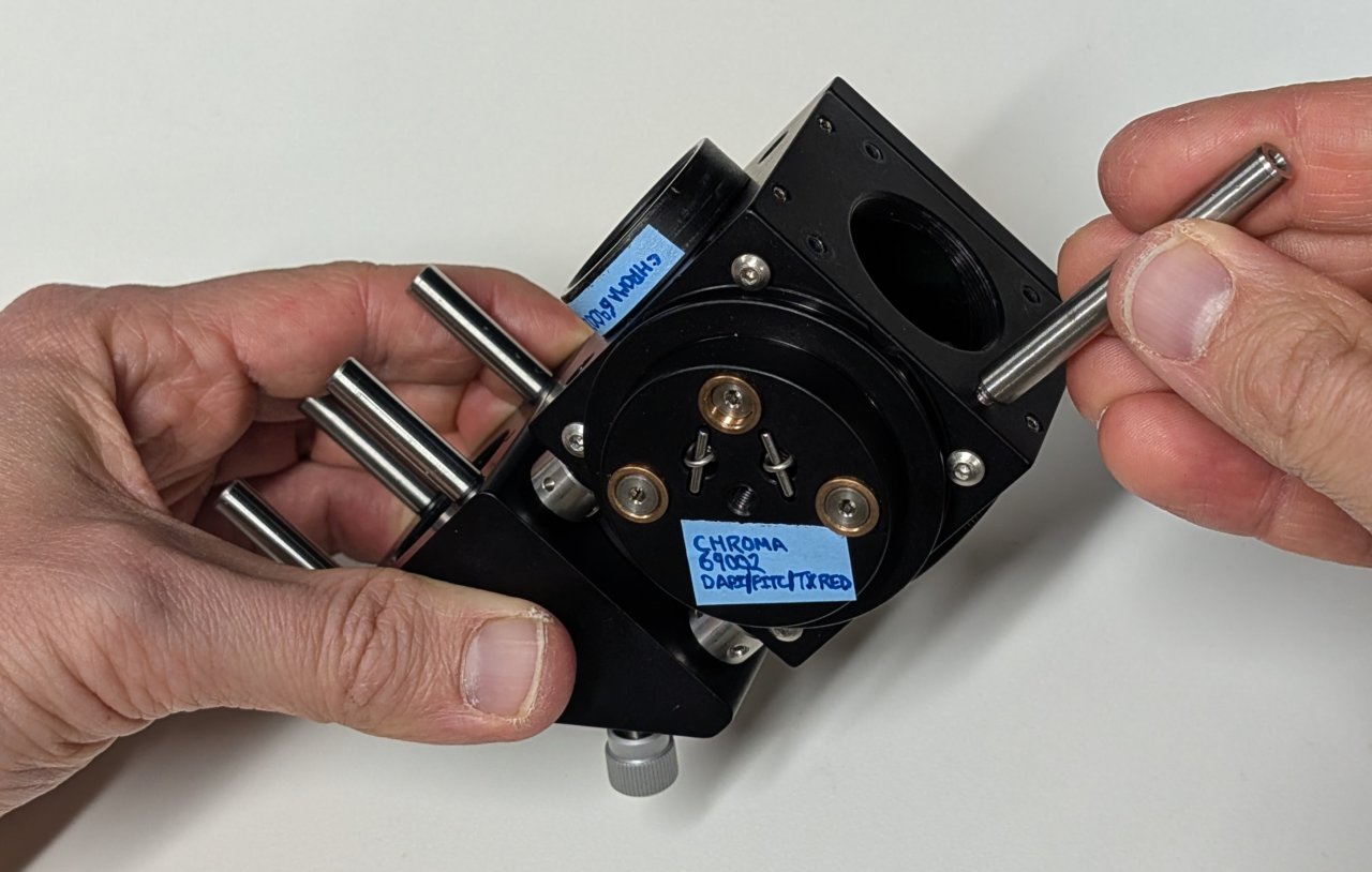
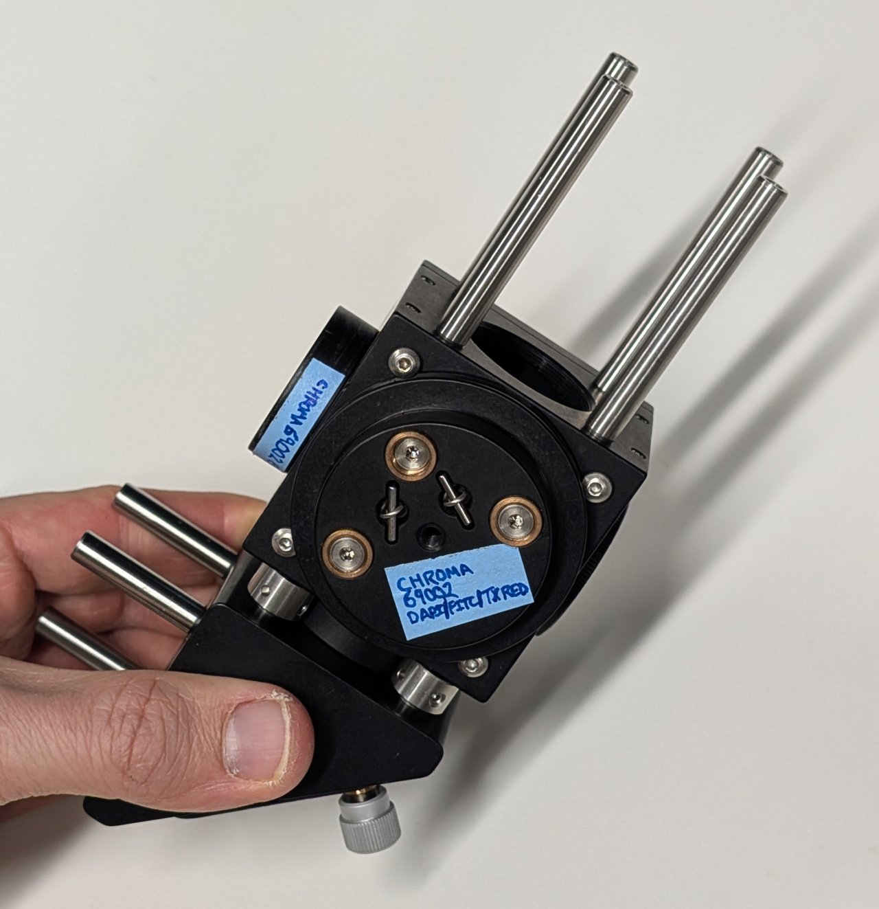
9
Slide the slip plate onto the ends of the cage rods. Lock it into place with the set screws.
10
Attach the cage system covers to the four sides of the 2“ cage rod subassembly.
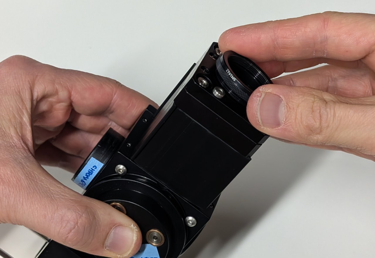
11
Insert the SM1 to M25 thread adapter into the slip plate.
12
Thread pedestals into the bottoms of the two 30 mm long post holders.
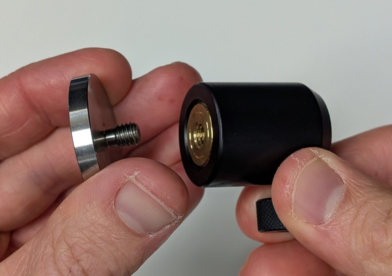
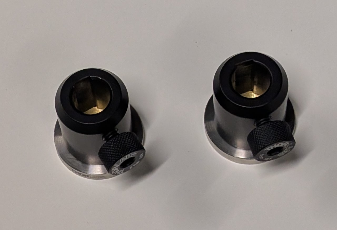
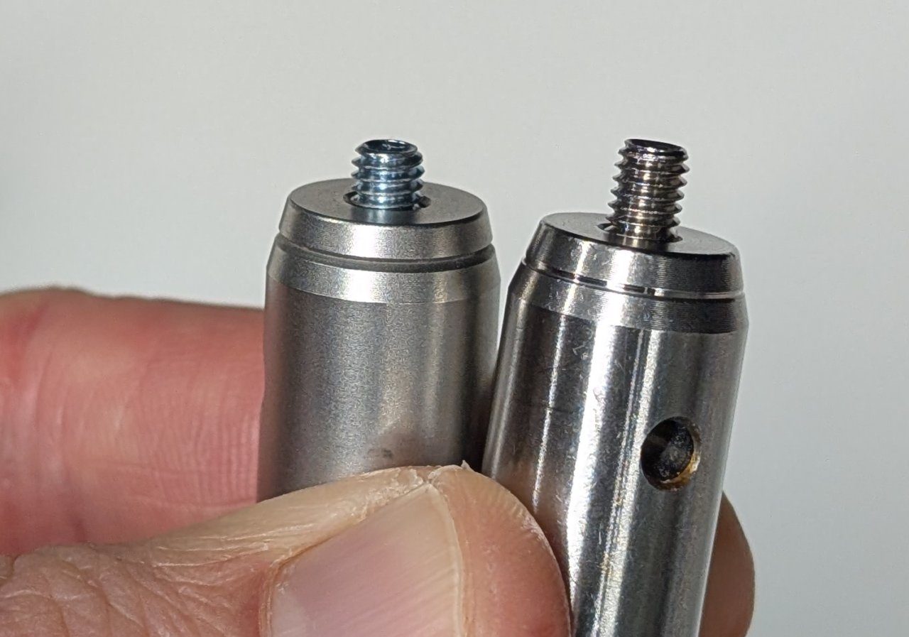
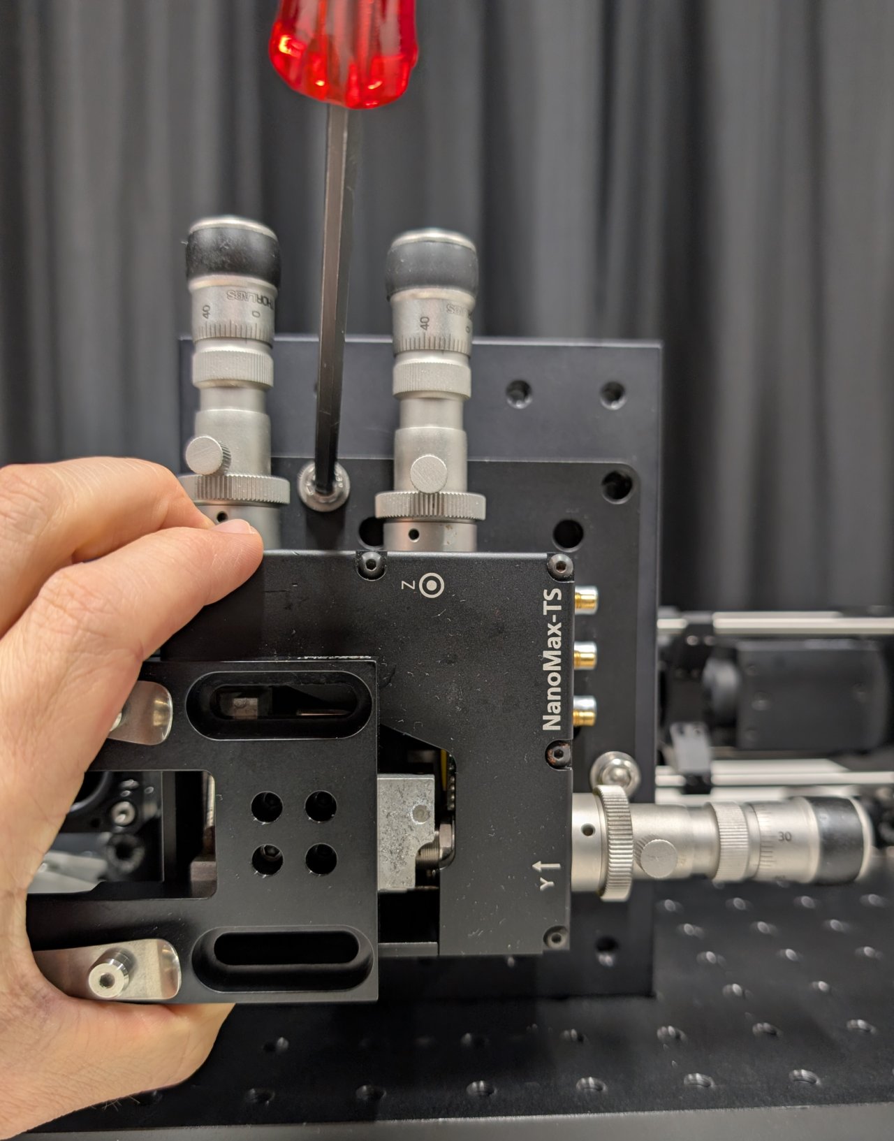
13
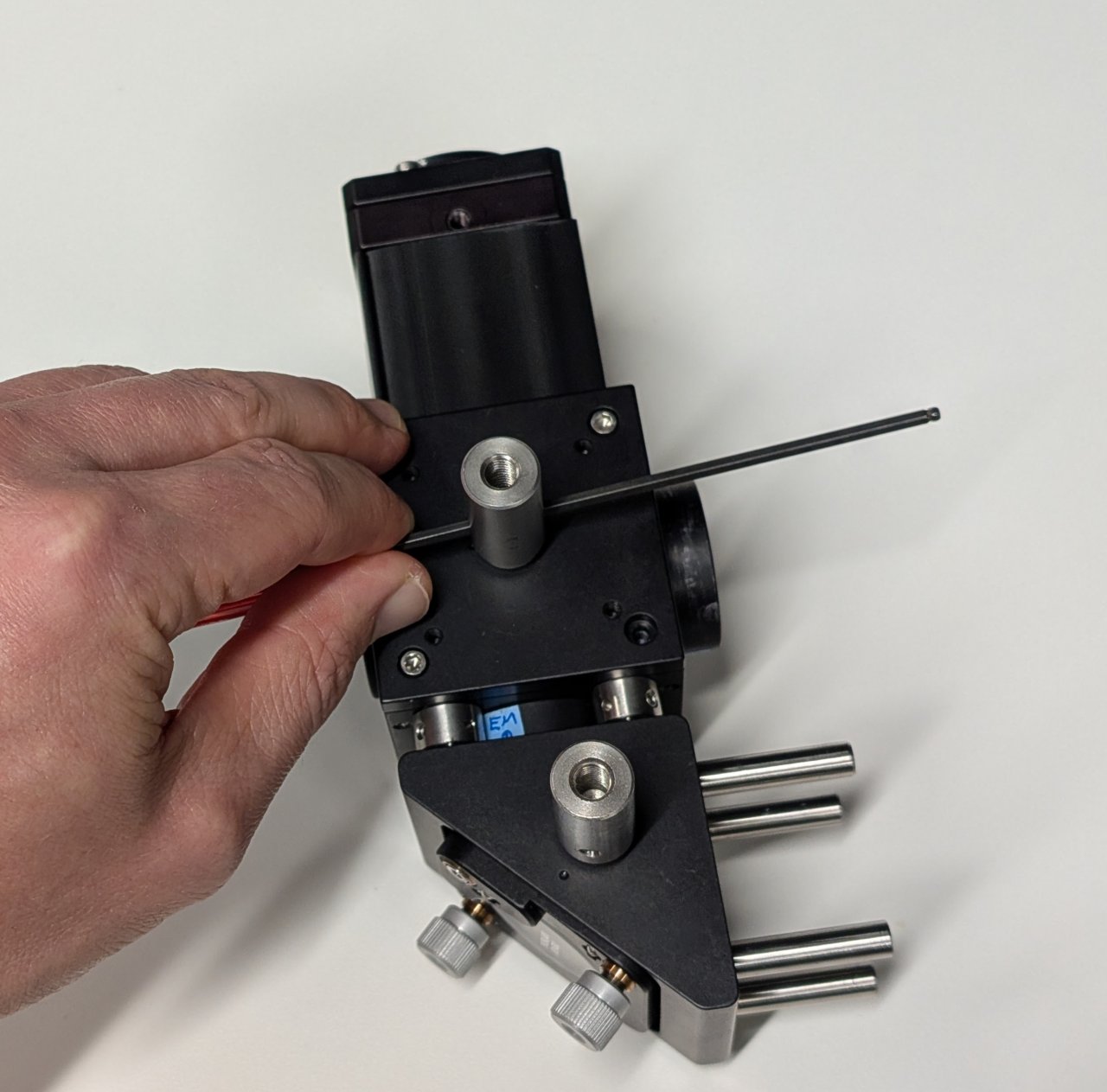
Note that one set screw is shorter than the other in the two, 30 mm long posts.
Attach the one with the shorter set screw to the bottom of the cage cube. Attach the other to the bottom of the right-angle mirror mount.
Use a hex driver and the post hole to lightly tighten the posts.
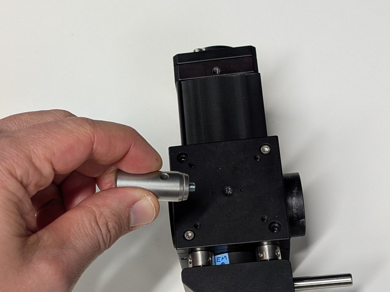
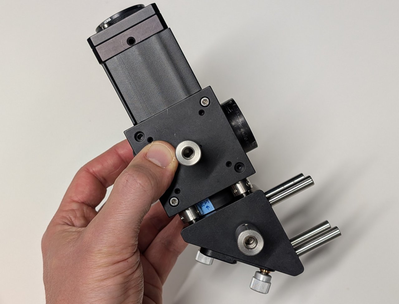
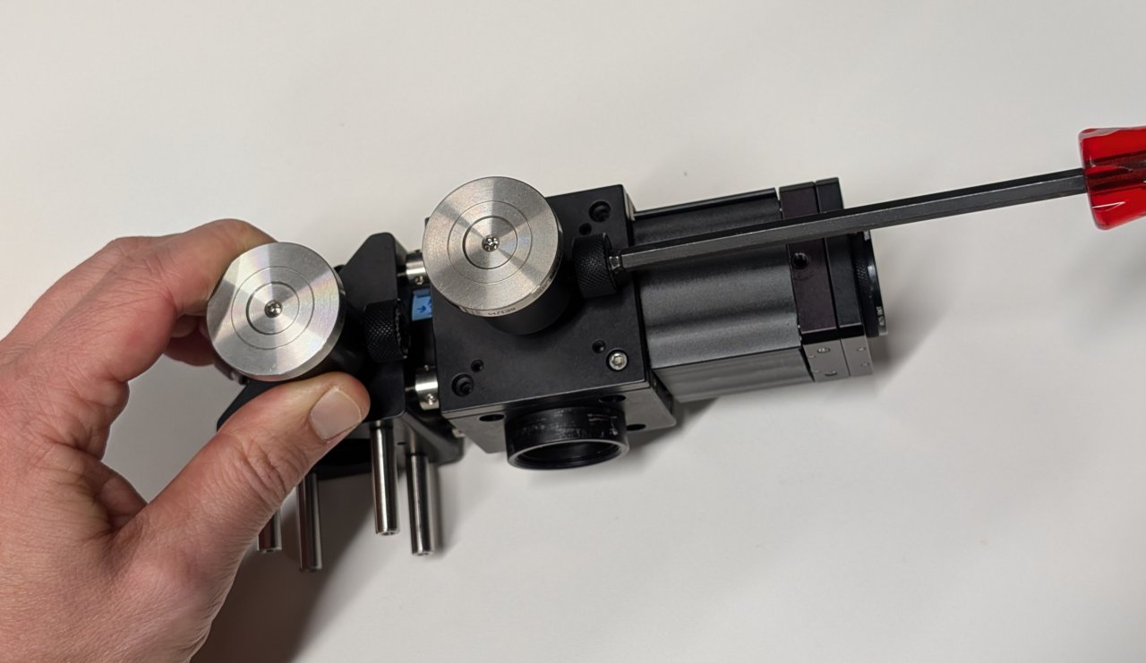
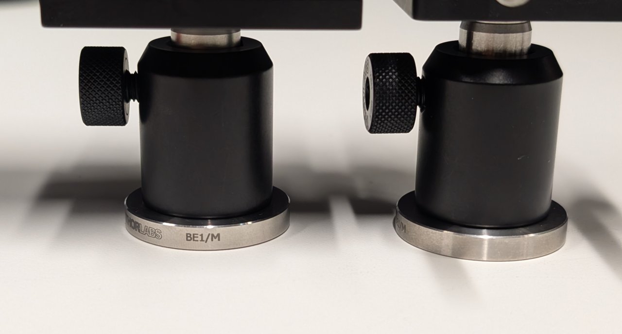
14
Attach the post holders to the posts.
Make sure that they are at the same height by placing the assembly on a flat surface and checking for any tilt.
15
Attach the 20 mm long post to the bottom of the cage plate of the camera and tube lens assembly.
Not shown: Slide on a 20 mm long post holder with a pedestal attached.
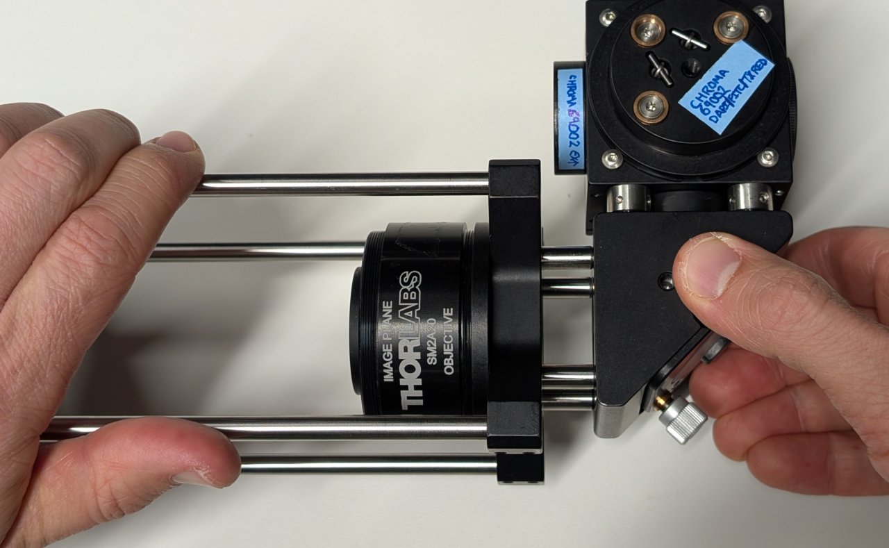
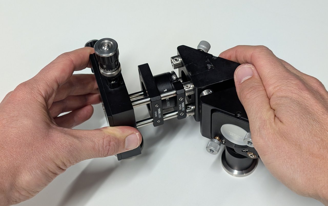
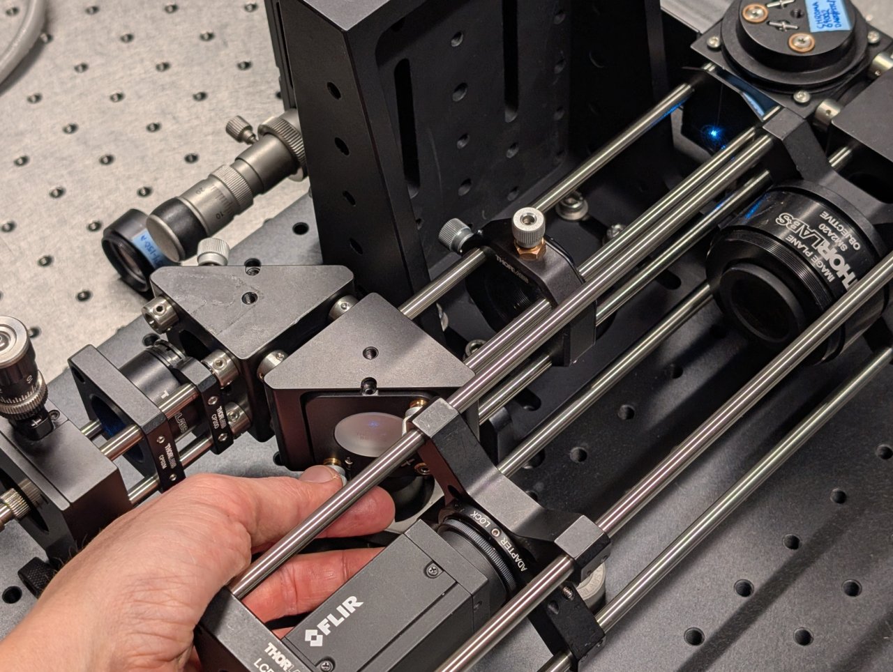
16
Slide the 30 mm to 60 mm cage adapter from the tube lens/camera assembly onto the 30 mm cage rods of the right-angle mirror.
Tighten the set screws to join the two assemblies together.
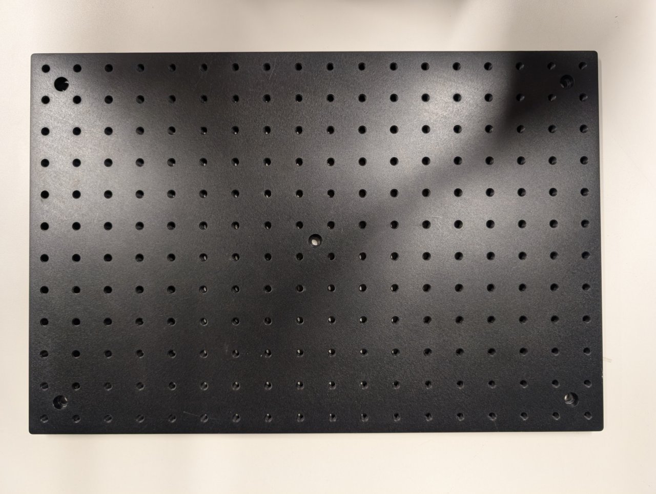
17
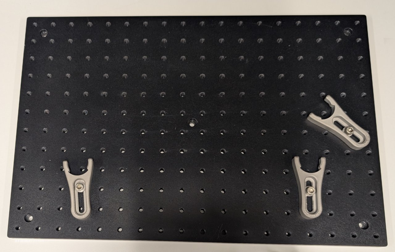
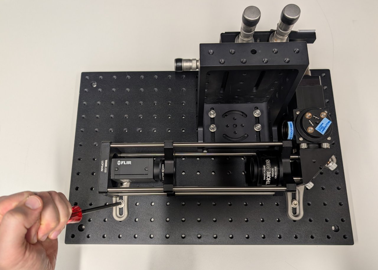
Let \( ( \text{row} \, , \text{col} ) \) denote the row and column coordinates of a screw hole on the base plate. Take the upper left hole of the base plate as the origin (0, 0), with the row coordinate increasing downward and the column coordinate increasing to the right. Do not take the counterbored holes into consideration.
Place the screws for the three clamping forks at the coordinates
| row | col |
|---|---|
| 9 | 3 |
| 6 | 16 |
| 9 | 14 |
18
Slide the pedestals into the clamping forks. Do not tighten them yet.
19
Attach the large right-angle bracket to the base plate as shown using the following screw holes:
| row | col |
|---|---|
| 3 | 9 |
| 4 | 9 |
| 3 | 12 |
| 4 | 12 |
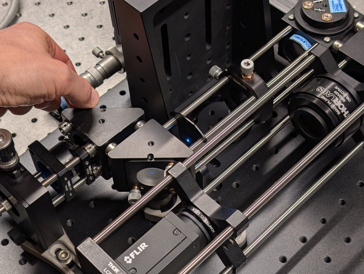
20
Attach the sample positioner to the top of the right-angle bracket.
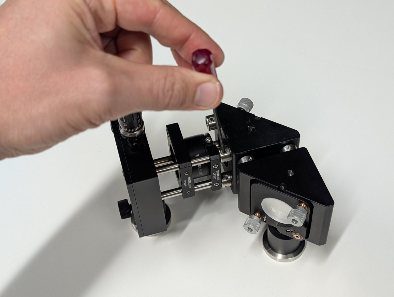
21
Carefully screw the objective into the SM1 to M25 thread adapter.
22
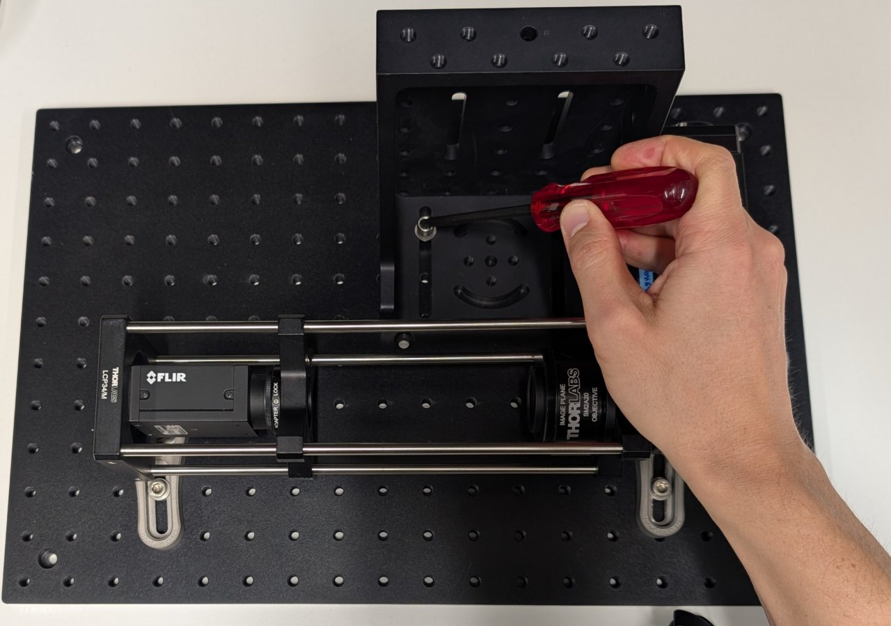
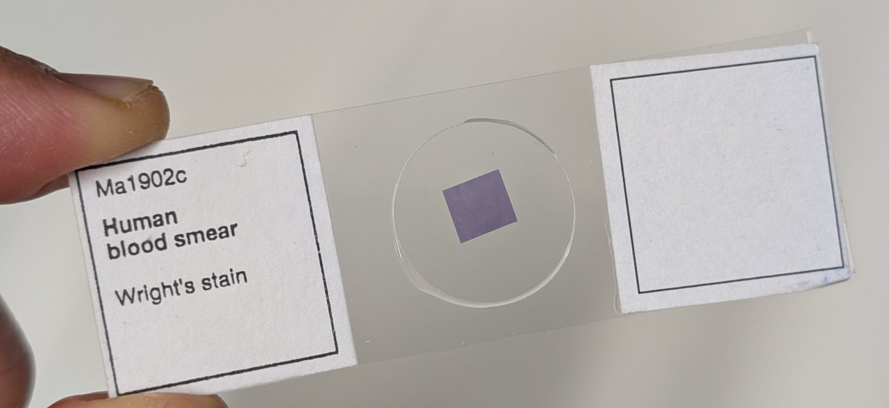
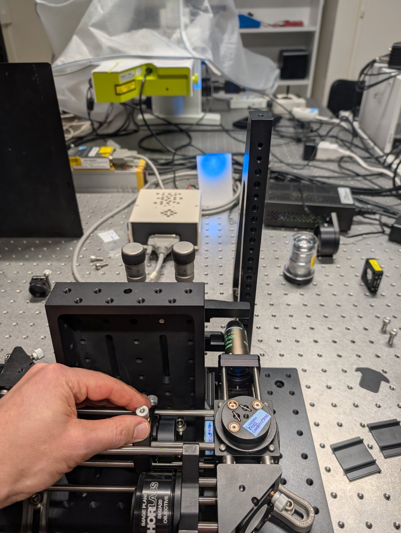
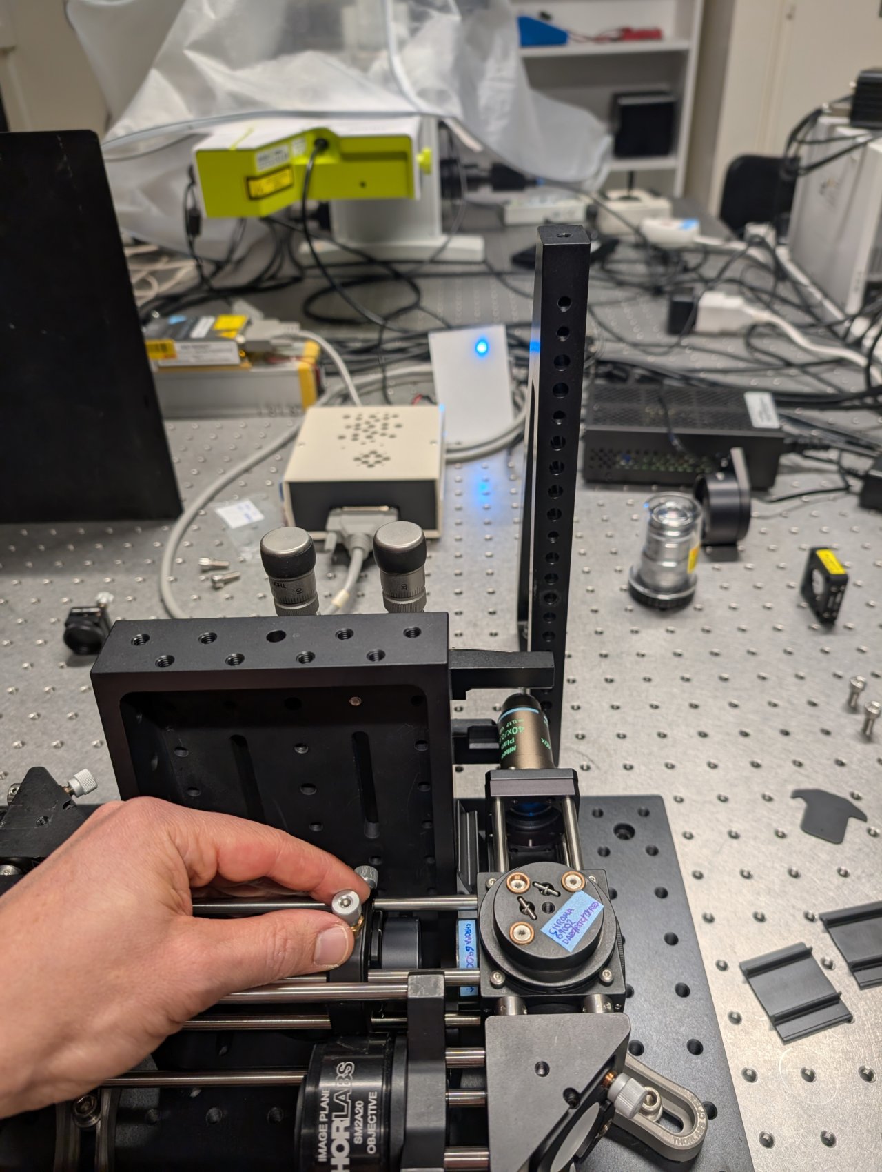
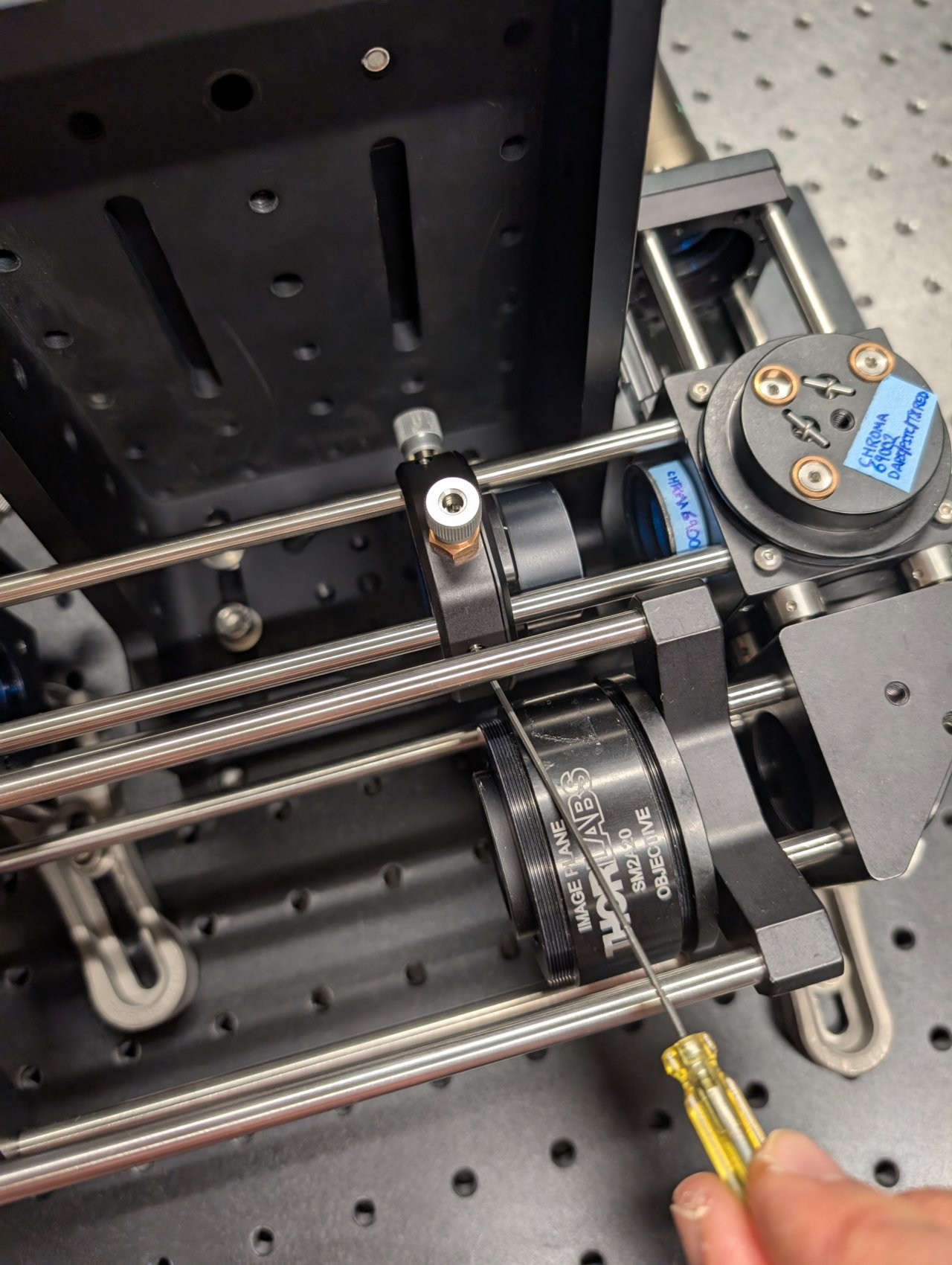
Place a slide with an easy-to-see sample, such as a blood smear, onto the sample holder. Check its position relative to the objective.
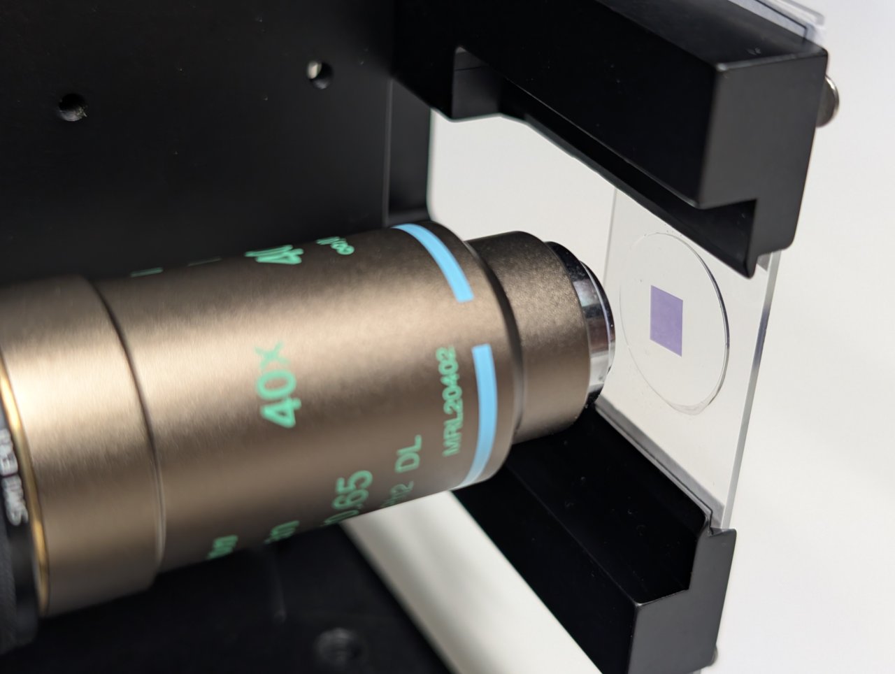
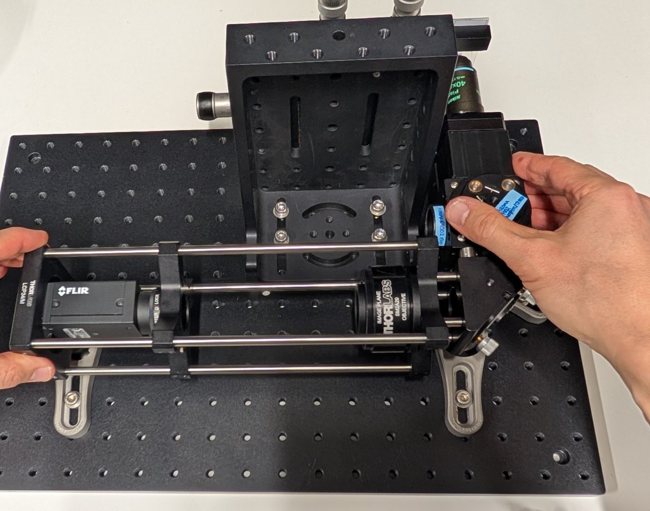
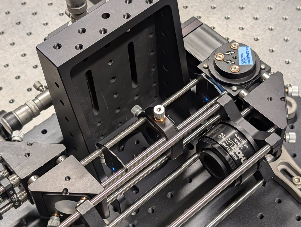
23
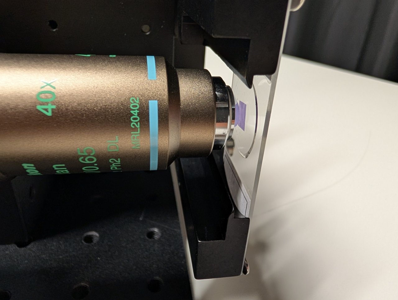
Gently and carefully move the entire microscope assembly to position the sample approximately 1 or 2 mm from the end of the objective.
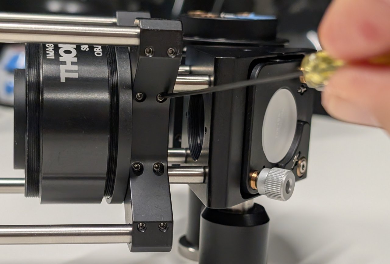
Make sure that the holes for the cage rods on the cage cube are not blocked by the right-angle bracket.
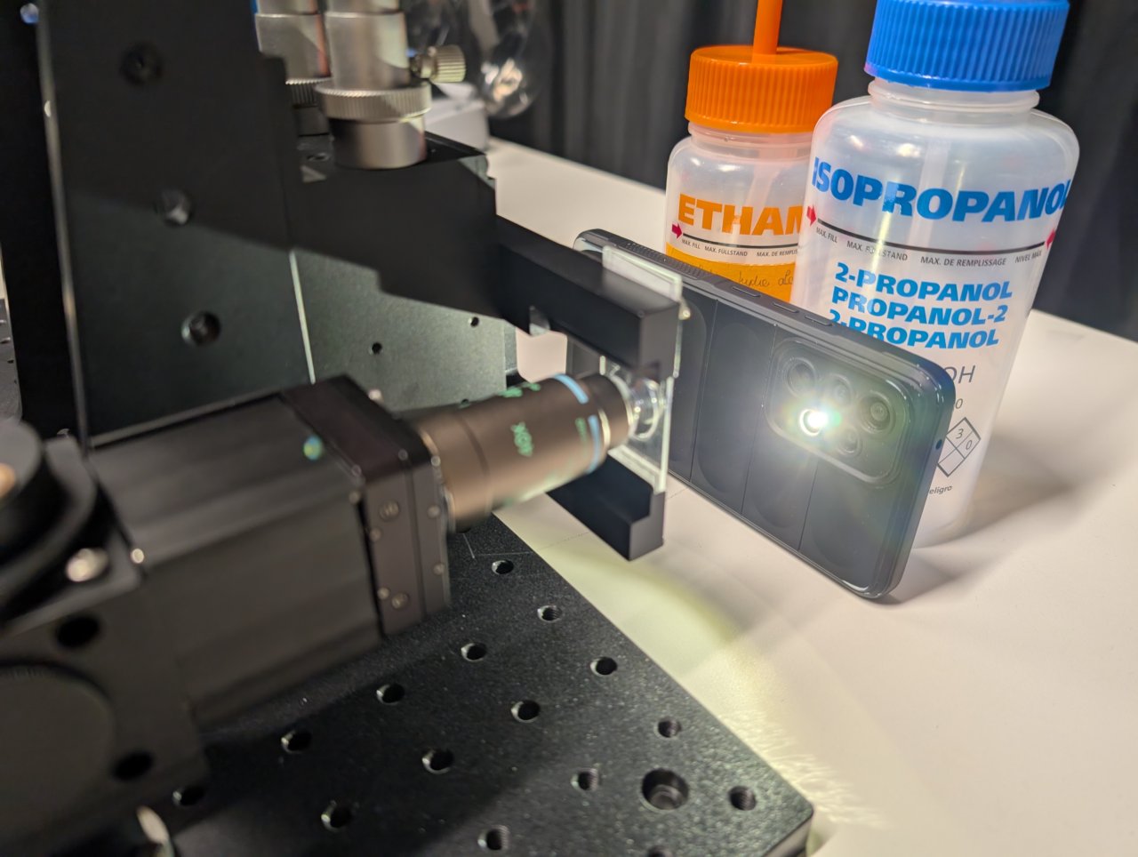
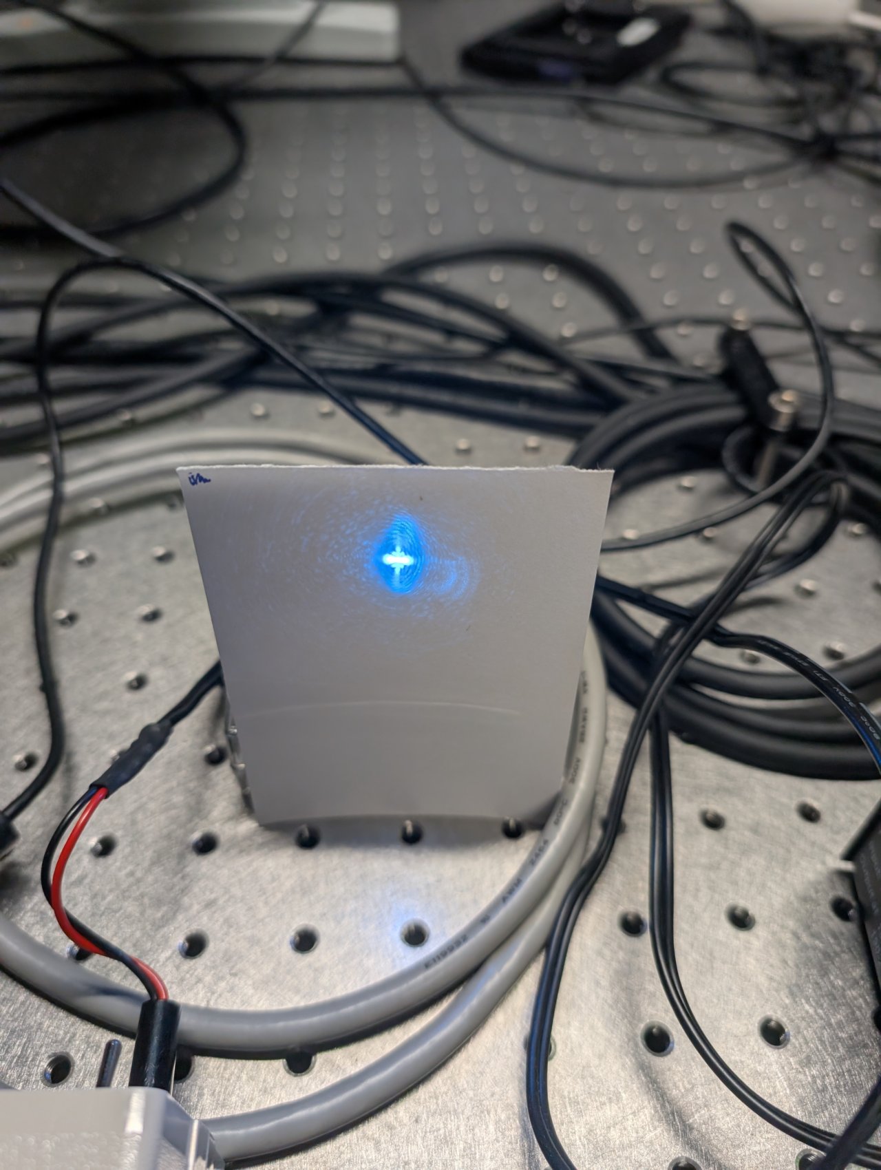
24
Put a smartphone with a flashlight in front of the sample. Connect the camera to the PC and start a live acquisition.
Further adjust the microscope assembly until the image is in focus.
It is OK if the image contrast and quality is poor at this point. Just try to make it in focus.
Not shown: Adjust the screws on the right-angle mirror mount if the image is not centered on the camera.
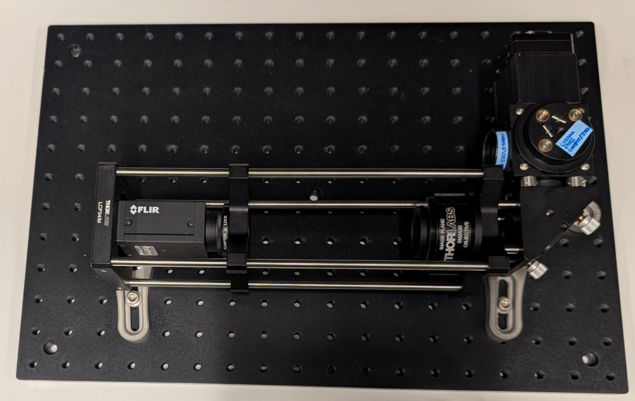
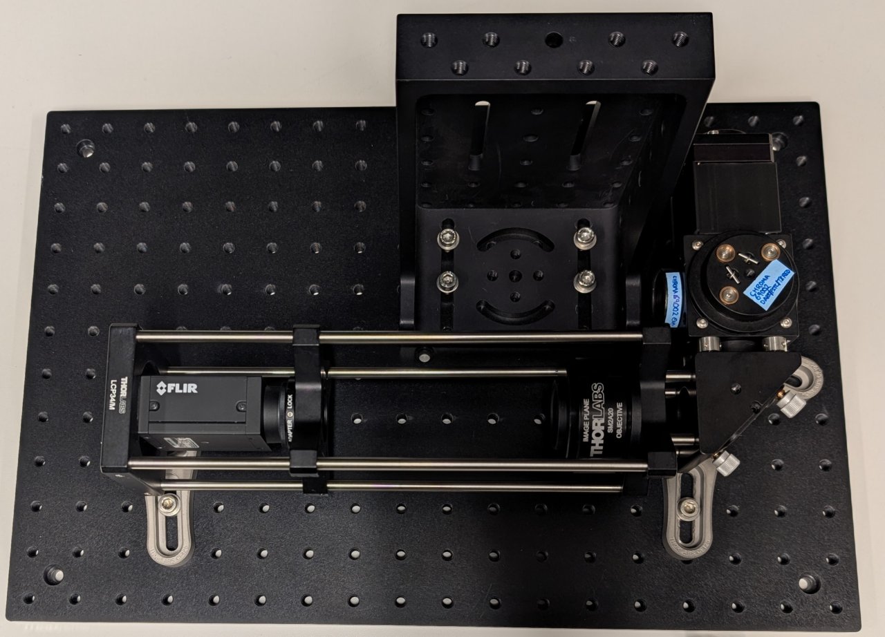
25
Tighten all screws to secure the assembly to the base plate.
Control the Laser
Construct the Microscope Excitation Path
Parts List
Below is the parts list for this section of the basic training course. Note that some of the parts used in the course are now obsolete. In these cases the parts listed below are the closest current match to the obsolete parts.
| Part | Manf. Part No. | Quantity | URL |
|---|---|---|---|
| f=45 mm, Ø1“ Achromatic Doublet, SM1-Threaded Mount, ARC: 400-700 nm | AC254-045-A-ML | 1 | https://www.thorlabs.com/thorproduct.cfm?partnumber=AC254-045-A-ML |
| f=150 mm, Ø1“ Achromatic Doublet, SM1-Threaded Mount, ARC: 400-700 nm | AC254-150-A-ML | 1 | https://www.thorlabs.com/thorproduct.cfm?partnumber=AC254-150-A-ML |
| Ø1“ Broadband Dielectric Mirror, 400 - 750 nm | BB1-E02 | 2 | https://www.thorlabs.com/thorproduct.cfm?partnumber=BB1-E02 |
| FC/PC Fiber Adapter Plate with External SM1 (1.035“-40) Threads, Narrow Key (2.0 mm) | SM1FC2 | 1 | https://www.thorlabs.com/thorproduct.cfm?partnumber=SM1FC2 |
| XY Translator with Differential Drives, Metric | ST1XY-D/M | 1 | https://www.thorlabs.com/thorproduct.cfm?partnumber=ST1XY-D/M |
| Right-Angle Kinematic Mirror Mount with Tapped Cage Rod Holes, 30 mm Cage System and SM1 Compatible, M4 and M6 Mounting Holes | KCB1/M | 2 | https://www.thorlabs.com/thorproduct.cfm?partnumber=KCB1/M |
| 30 mm Cage System, XY Translating Lens Mount for Ø1“ Optics | CXY1A | 1 | https://www.thorlabs.com/thorproduct.cfm?partnumber=CXY1A |
| 30 mm Cage System Iris Diaphragm (Ø0.8 - Ø20 mm) | CP20D | 1 | https://www.thorlabs.com/thorproduct.cfm?partnumber=CP20D |
| SM1-Threaded 30 mm Cage Plate, 0.35“ Thick, 2 Retaining Rings, M4 Tap | CP33/M | 1 | https://www.thorlabs.com/thorproduct.cfm?partnumber=CP33/M |
| Rod Adapter for Ø6 mm ER Rods, L = 0.27“ | ERSCB | 8 | https://www.thorlabs.com/thorproduct.cfm?partnumber=ERSCB |
| Cage Assembly Rod, 1/4“ Long, Ø6 mm | ER025 | 4 | https://www.thorlabs.com/thorproduct.cfm?partnumber=ER025 |
| Cage Assembly Rod, 2“ Long, Ø6 mm | ER2 | 3 | https://www.thorlabs.com/thorproduct.cfm?partnumber=ER2 |
| Cage Assembly Rod, 6“ Long, Ø6 mm | ER6 | 3 | https://www.thorlabs.com/thorproduct.cfm?partnumber=ER6 |
| Ø12.7 mm Optical Post, SS, M4 Setscrew, M6 Tap, L = 20 mm | TR20/M | 1 | https://www.thorlabs.com/thorproduct.cfm?partnumber=TR20/M |
| Ø12.7 mm Optical Post, SS, M4 Setscrew, M6 Tap, L = 30 mm | TR30/M | 2 | https://www.thorlabs.com/thorproduct.cfm?partnumber=TR30/M |
| Ø1/2“ Post Holder, Spring-Loaded Hex-Locking Thumbscrew, L = 1“ | PH1 | 2 | https://www.thorlabs.com/thorproduct.cfm?partnumber=PH1 |
| Ø31.8 mm Studded Pedestal Base Adapter, M6 Threads | BE1/M | 2 | https://www.thorlabs.com/thorproduct.cfm?partnumber=BE1/M |
| Clamping Fork for Ø1.25“ Pedestal Bases, 44.4 mm Counterbored Slot, M6 x 1.0 Captive Screw | CF175C/M | 2 | https://www.thorlabs.com/thorproduct.cfm?partnumber=CF175C/M |
Not shown: shear plate, CPA1 alignment plates.
Instructions
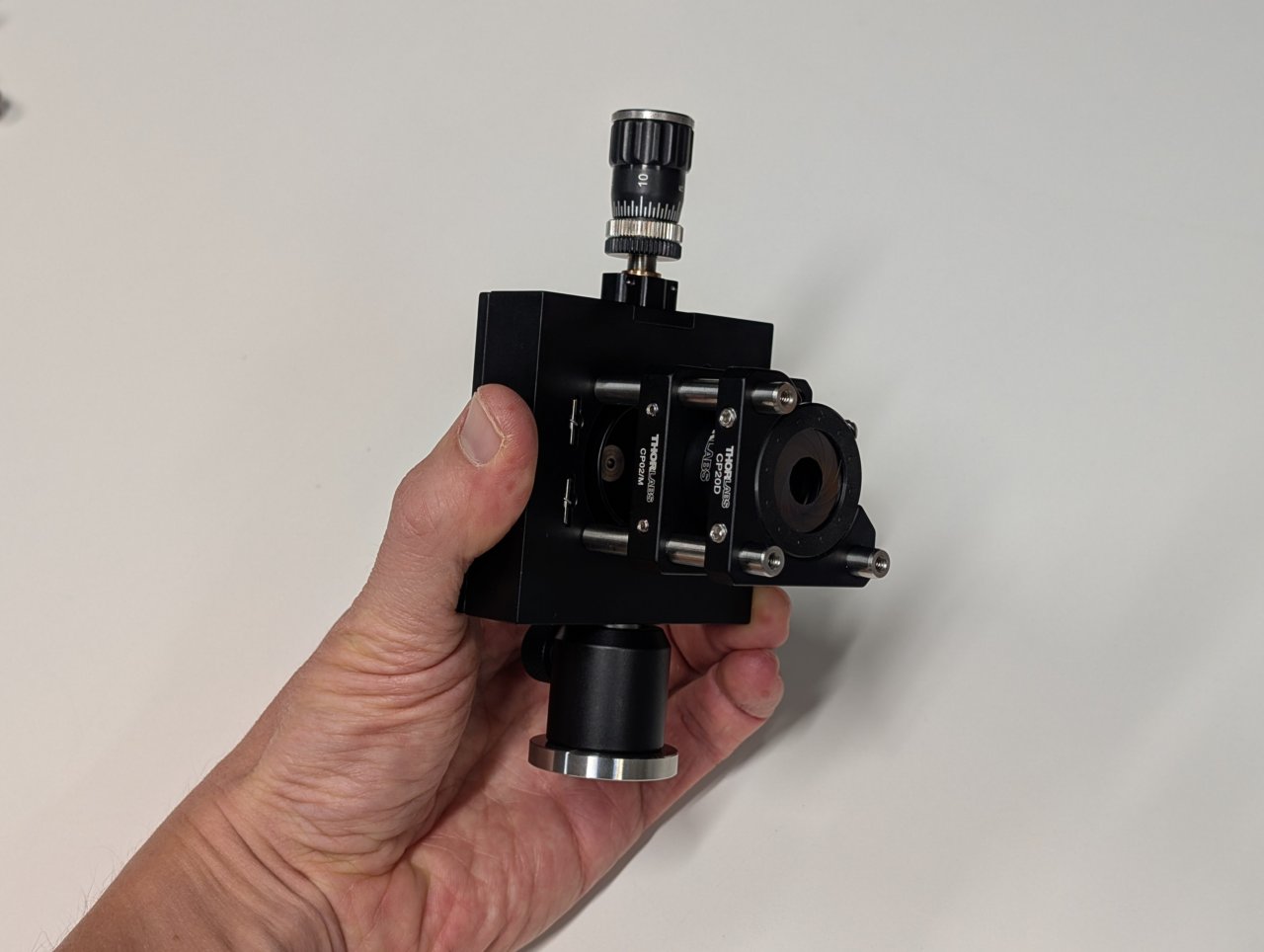
0
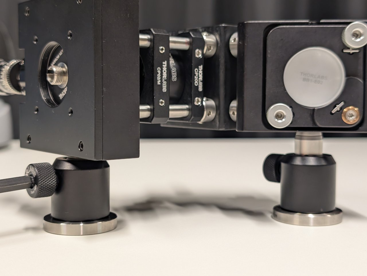
Thread the FC/PC fiber adapter plate into the XY transaltion mount such that it is recessed as far as the barrel’s internal amount will allow.
1
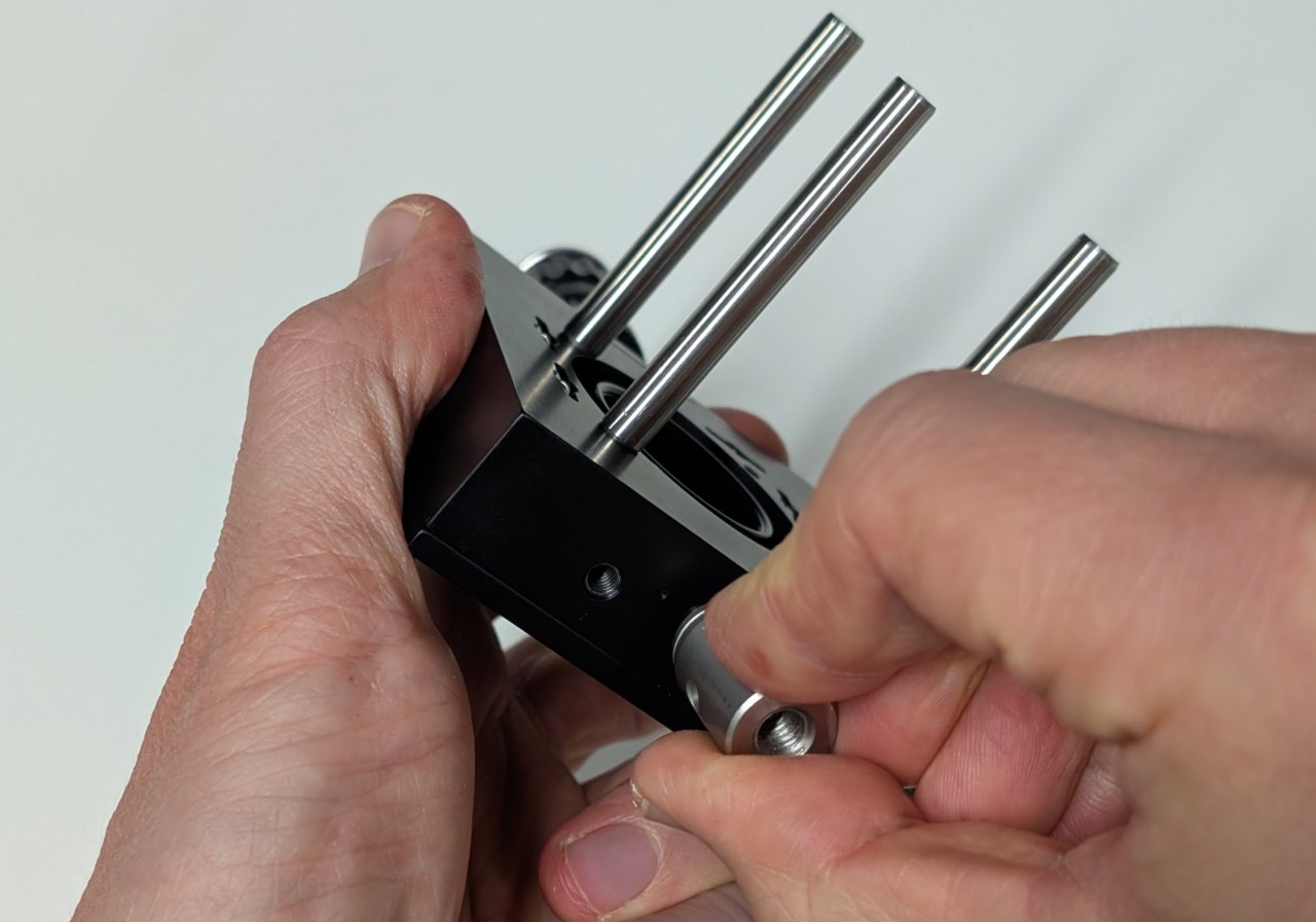
Attach three, 2“ cage rods to the translation mount in the manner shown in the photos. Leave one cage rod hole open for the iris that will be installed in a later step.
2
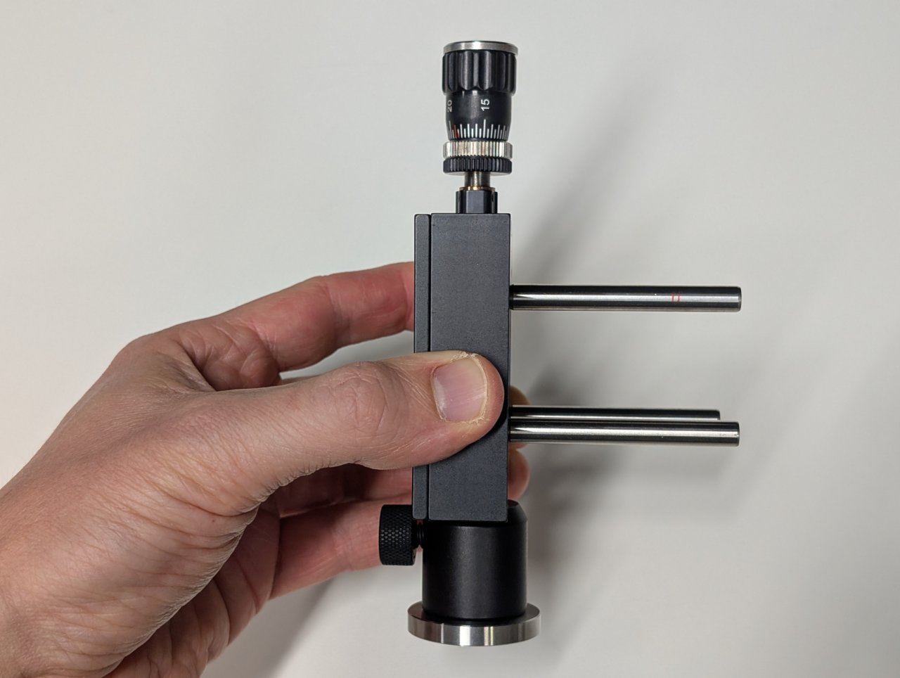
Attach a 20 mm post to the bottom of the translation mount. Insert it into a post holder and attach a pedestal base.
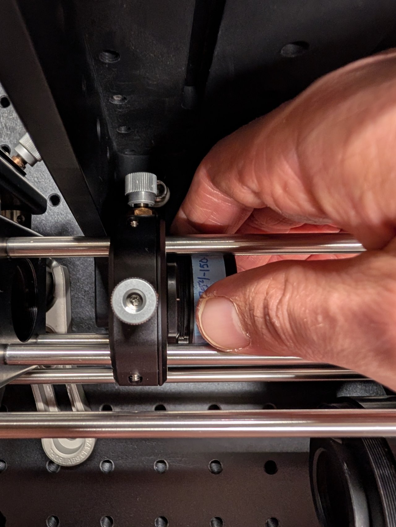
3
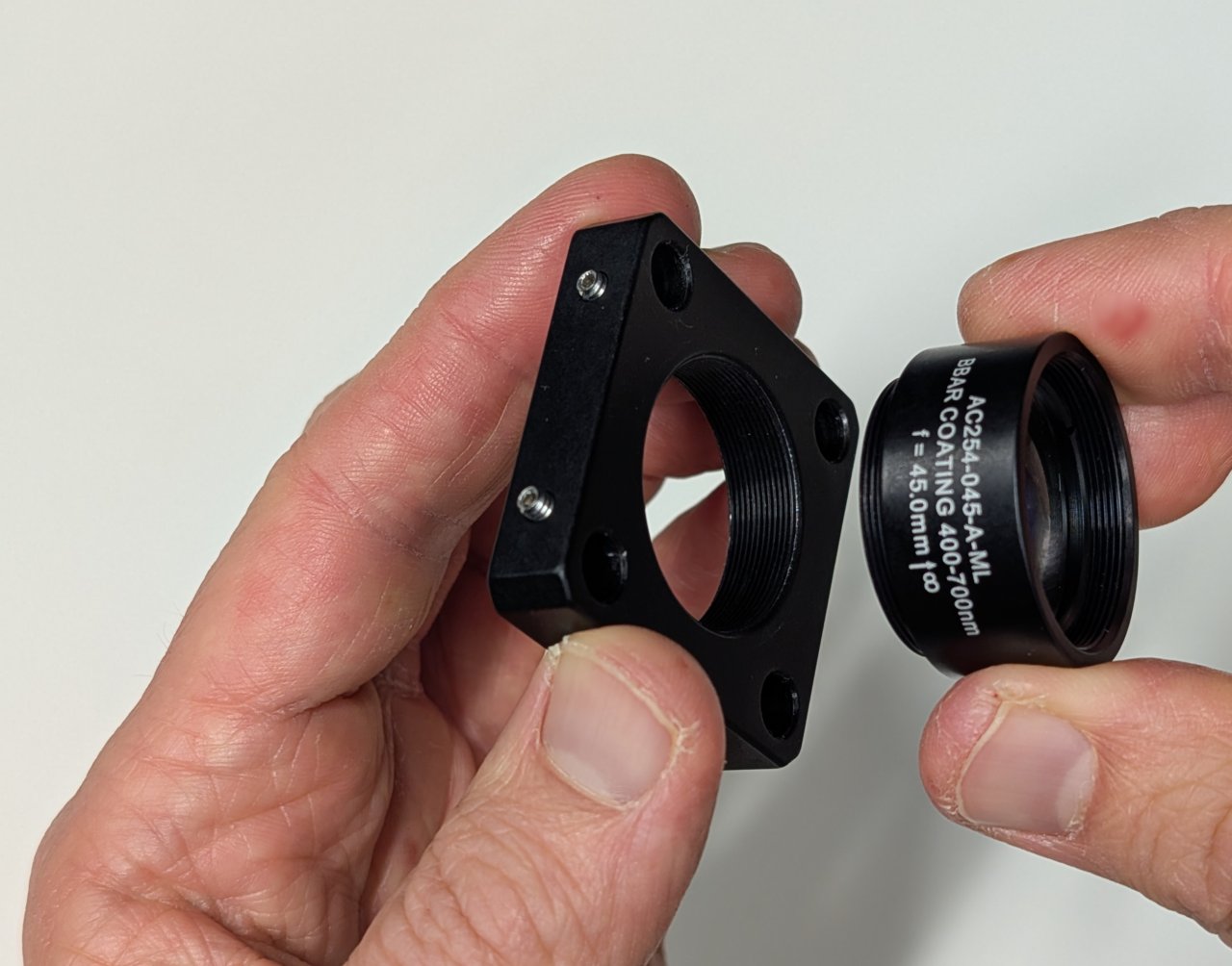
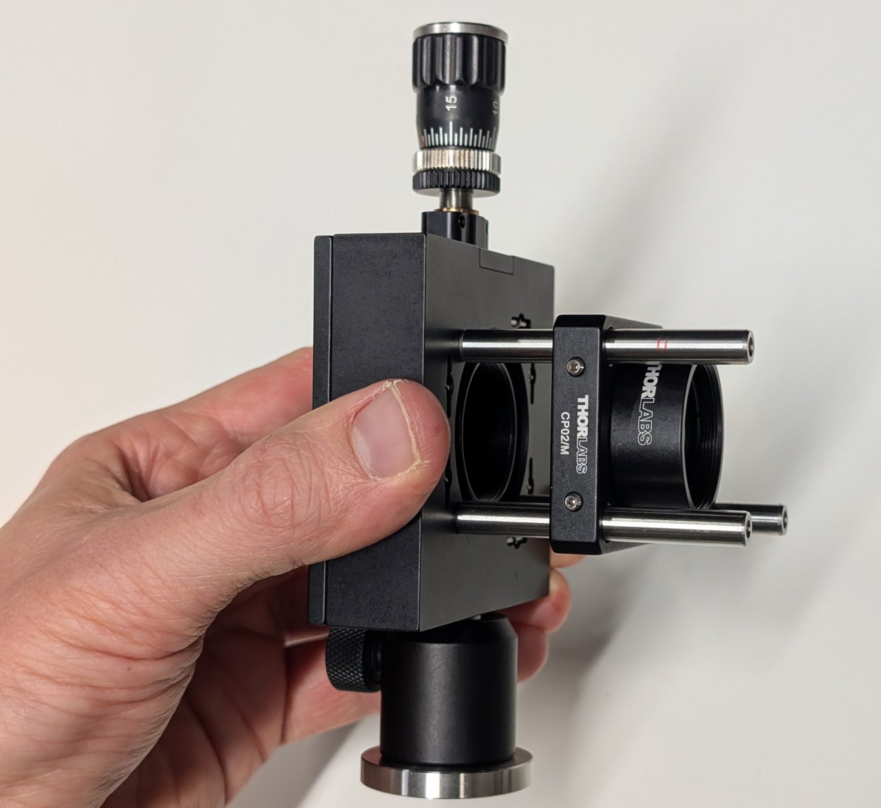
Thread the 45 mm achromat into the cage plate. Ensure that the direction marked as \( \infty \) points away from the fiber adapter plate.
Slide this assembly onto the cage rods.
Note the photo shows a CP02/M cage plate, but a CP33/M will work, too.
4
Attach the assembly to an optical table.
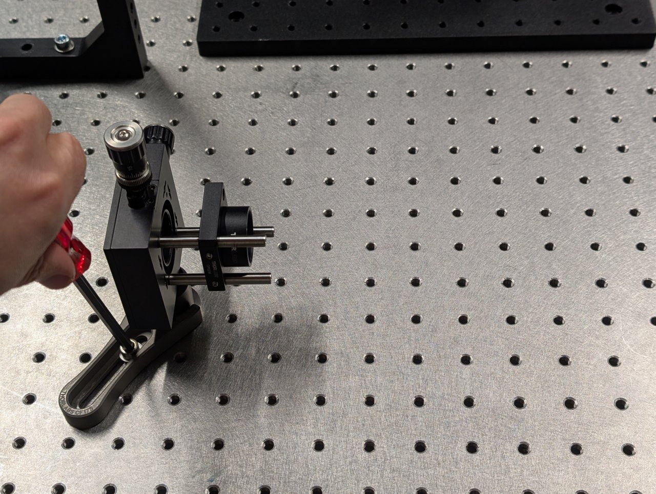
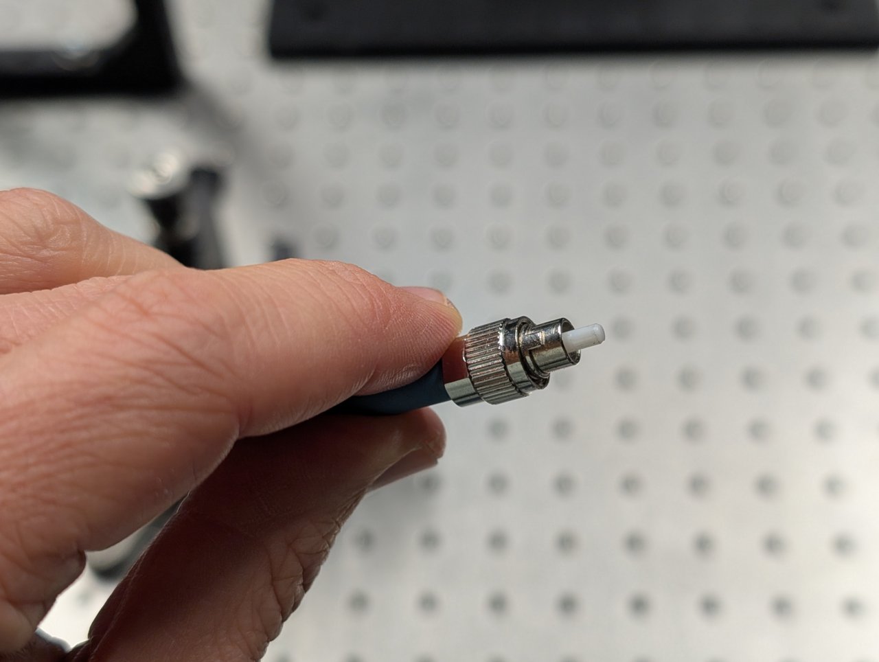
5
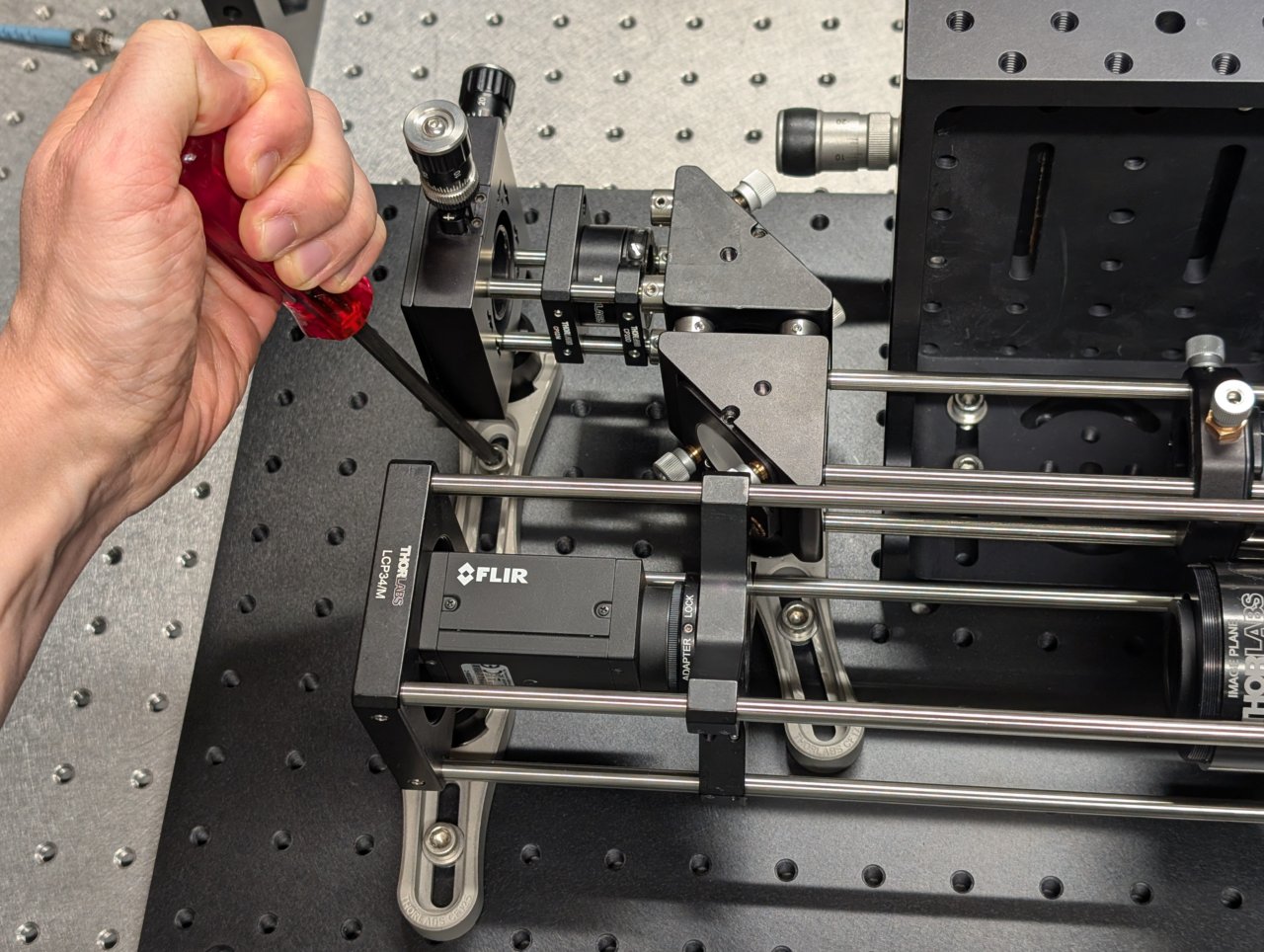
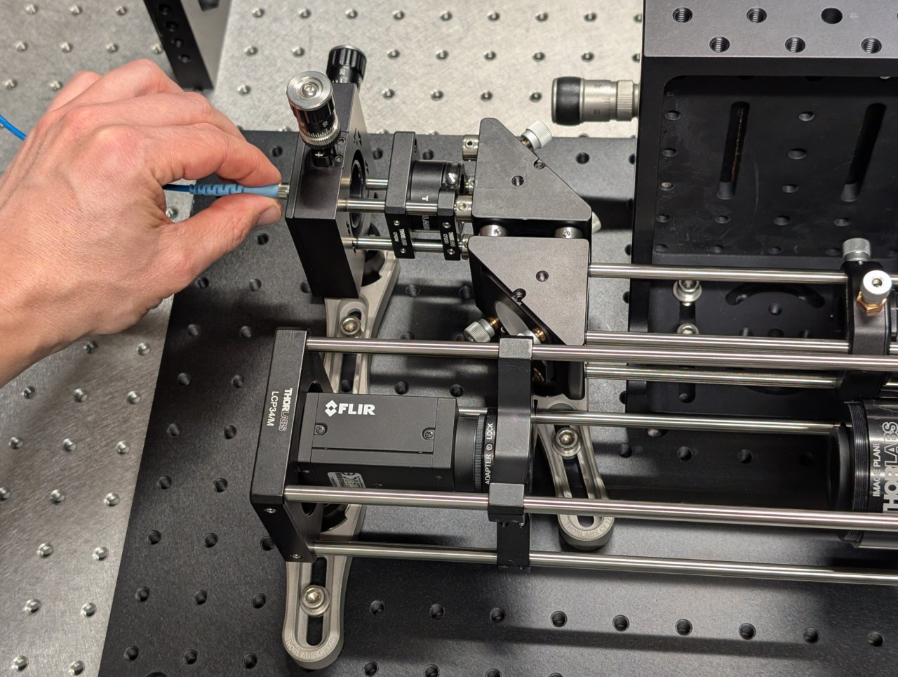
Attach the fiber from the laser engine (provided to you) to the fiber adapter plate. Ensure that the key on the fiber connector aligns with the notch on fiber adapter plate.
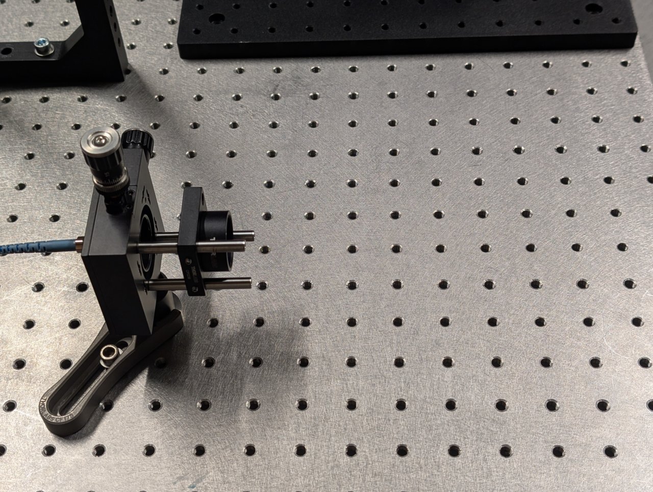
6
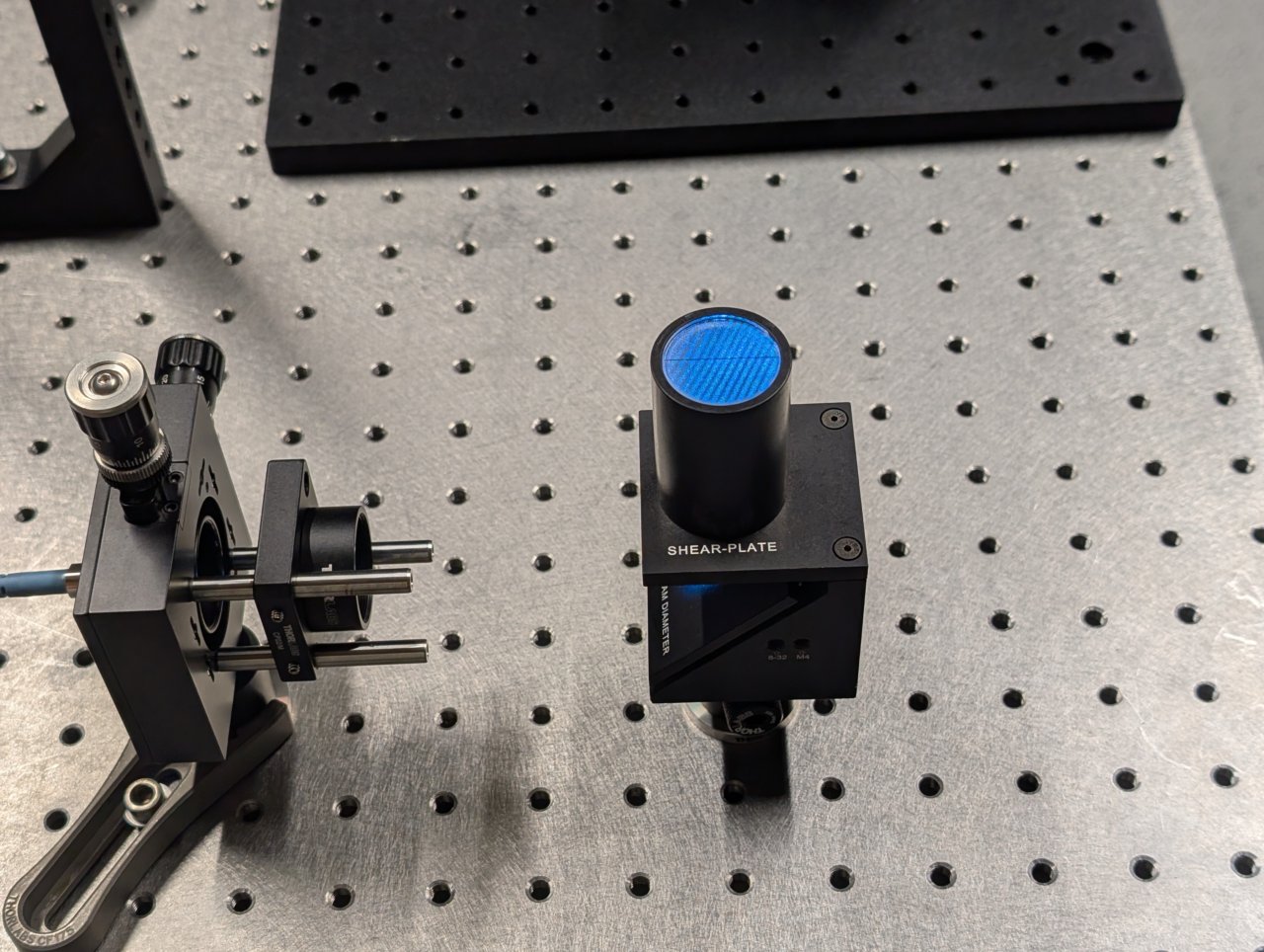
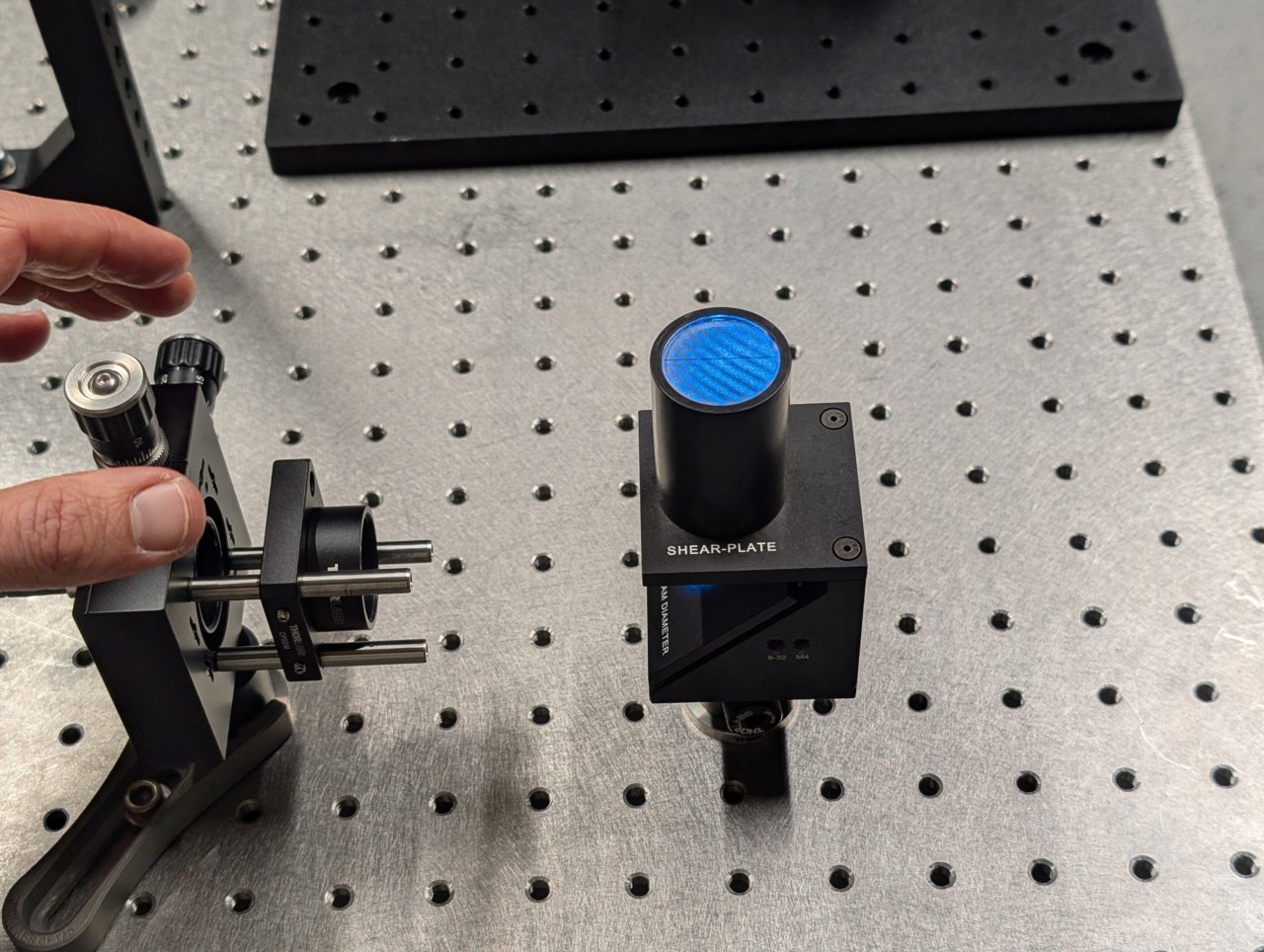
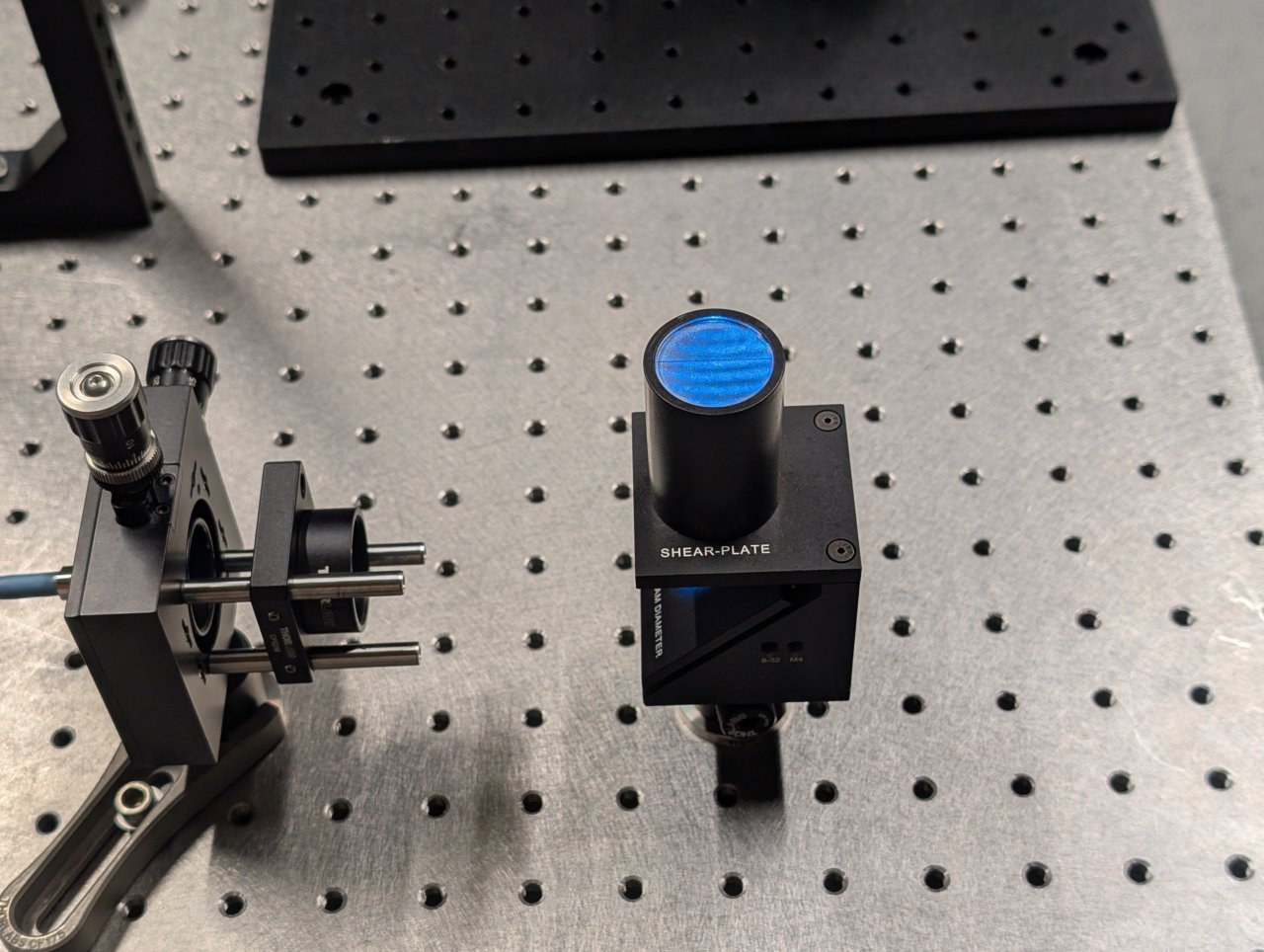
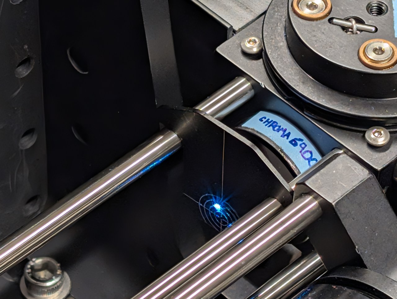
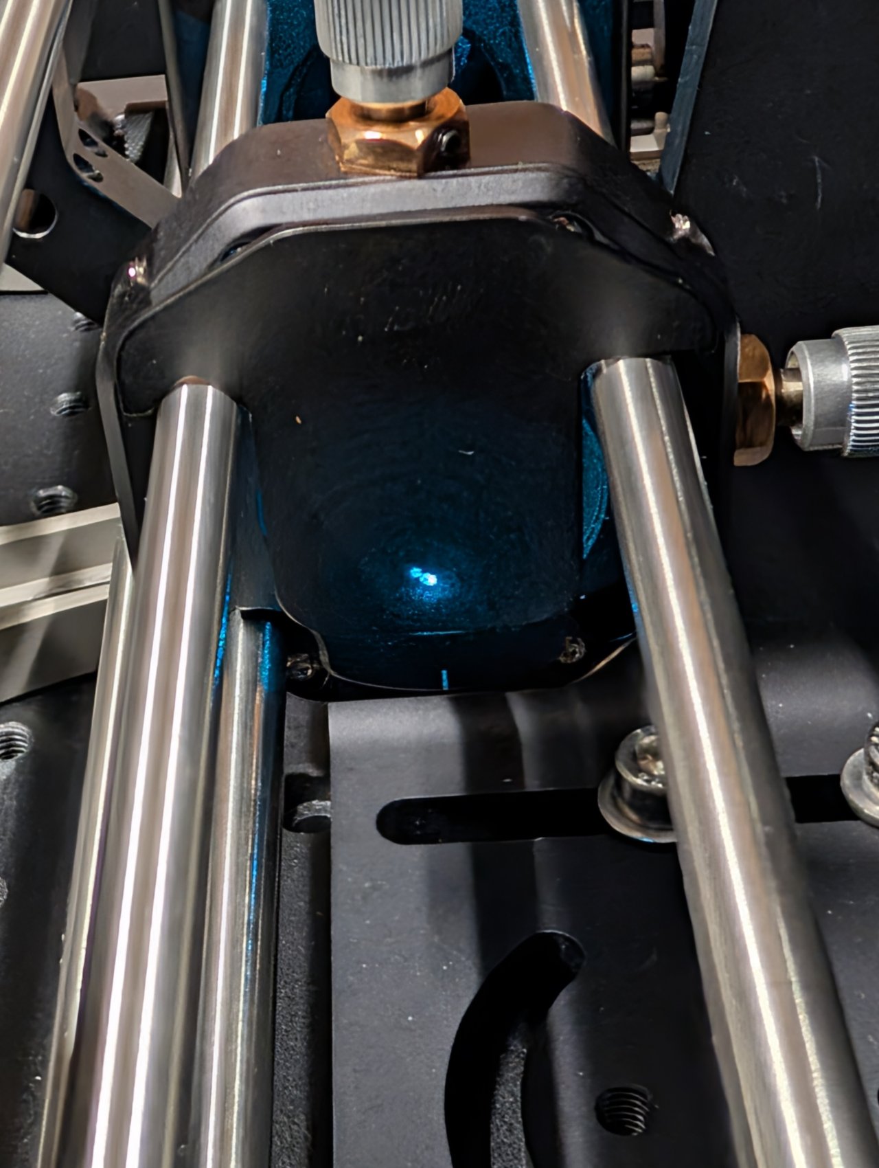
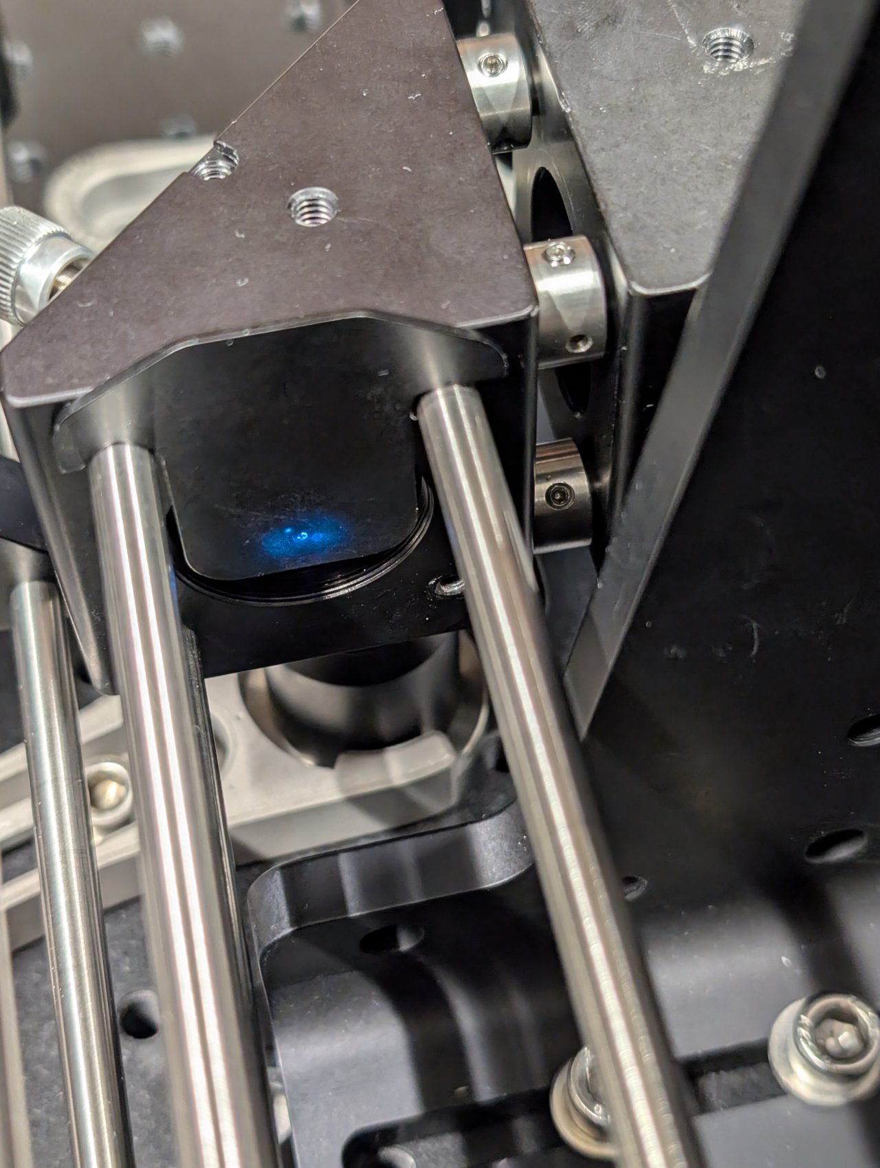
Turn on the laser. Position a shear plate in front of the laser beam.
Move the f = 45 mm lens in front of the fiber until the fringes on the shear plate are approximately parallel to the guideline.
The first two images below show the fringe pattern with the lens too close and too far from the fiber. The third image shows the lens position with the fiber in the focal plane of the lens.
Tighten the set screws on the cage plate once the correct position is found to lock it into place.
7
Slide the iris onto the end of the cage rods.
8
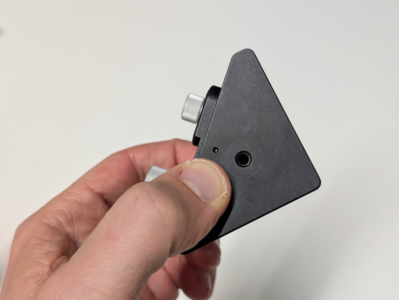
Note the dot on the bottom of the right-angle kinematic mirror mount.
We assume that there is a mirror already mounted inside the mount.
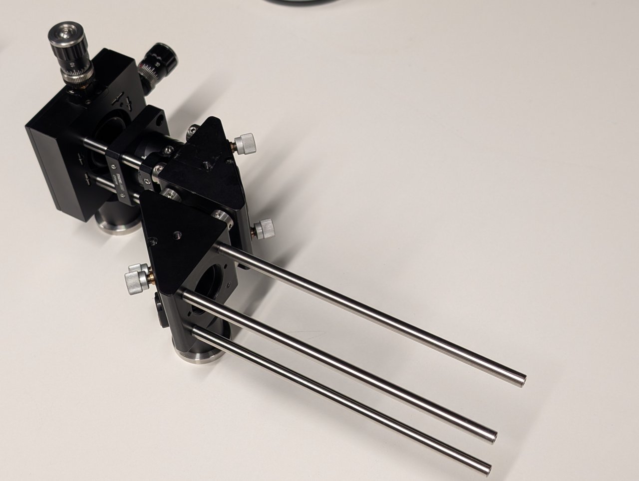
9
Attach four cage rod adapters to the mirror mount.
Metric cage rod adapters are shown, but imperial adapters work equally well.
10
Attach four, 0.25“ cage rods to the opposite side of the mirror mount.
Three cage rods are shown because that was all that we had when this photo was taken.
11
Attach cage rod adapters and the 30 mm post to the other right-angle kinematic mirror mount.
12
Attach a post holder with pedestal base to the mirror mount.
13
Attach one mirror mount to the other as shown using the cage rod adapters and 0.25“ cage rods.
14
Attach the fiber output coupler assembly to the steering mirrors assembly by inserting the 2“ cage rods into the other set of cage rod adapters.
15
Ensure that the assembly is level by checking the heights of the pedestals relative to the table. Adjust them if necessary.
16
Insert three, 6“ cage rods into the other end of the steering mirror assembly as shown.
Slide the XY translating lens mount onto the cage rods but do not tighten it yet.
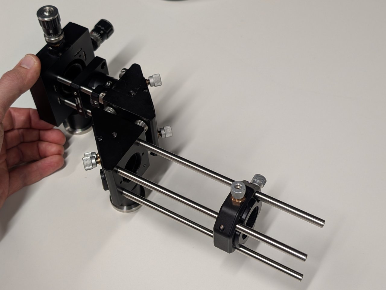
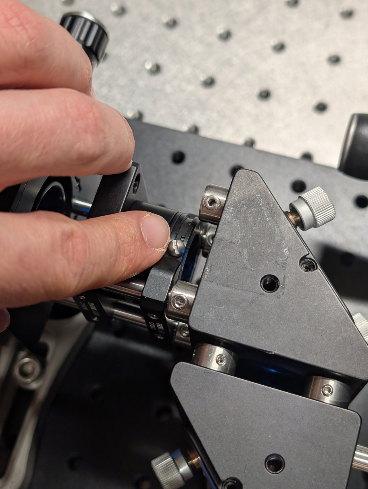
17
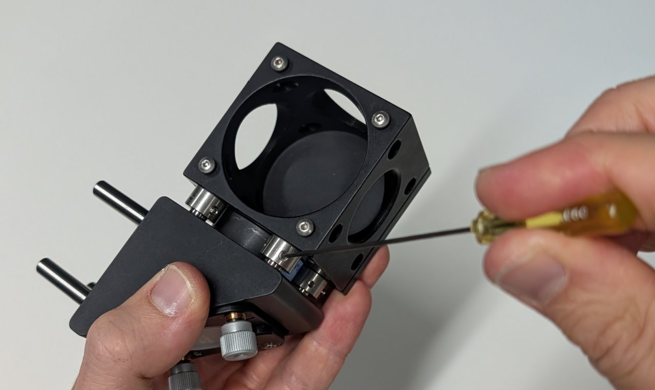
Slide the entire assembly into the cage rod holes in the dichroic cube, taking care not to damage the dichroic inside the mount. (It obstructs the cage rods from fully passing through the the cube.)
Not shown: Tighten the set screws that you can access with a hex driver.
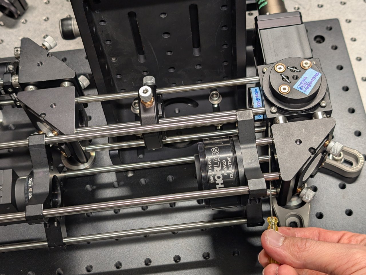
18
Use two clamping forks to attach the excitation path assembly to the base plate.
19
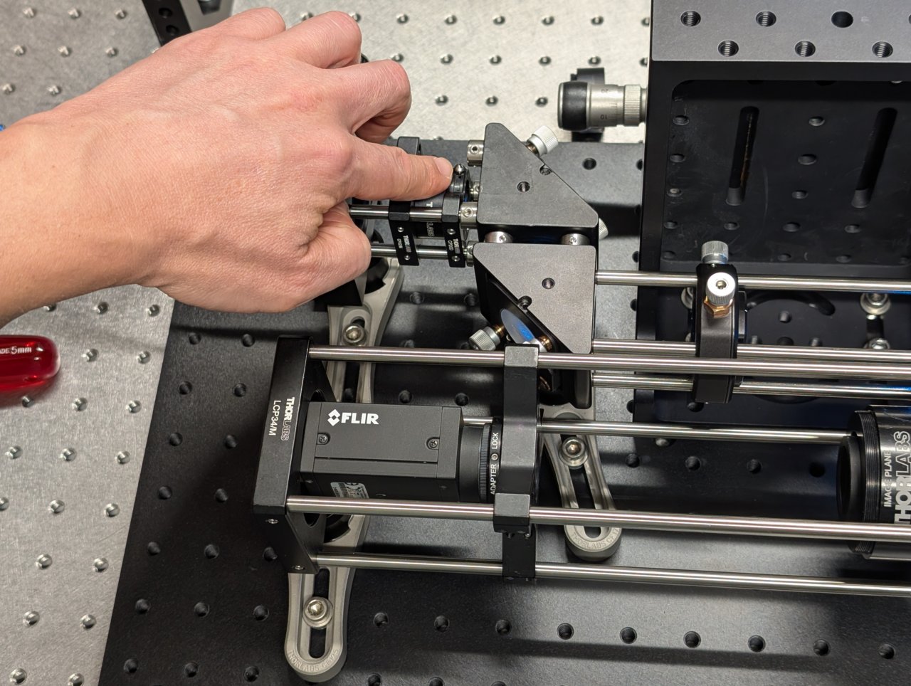
Attach the fiber to the fiber adapter plate.
20
Close the iris.
21
Turn on the laser and observe where the beam hits an alignment plate
- just before the excitation filter, and
- just after the beam steering mirrors.
The transverse beam positions measured at opposite ends of the cage rods tells you the beam location direction in 3D space.
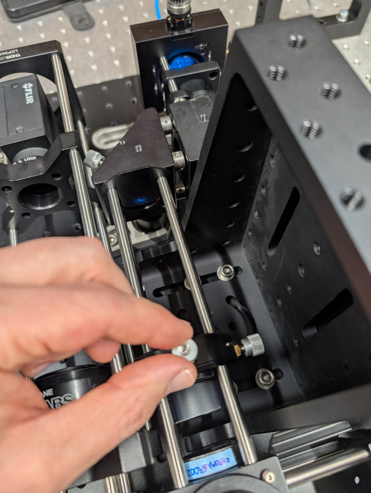
22
Align the laser beam to the center of the cage rods. Use the following procedure:
- Place the alignment plate at the end of the excitation path, just before the excitation filter.
- Turn the knobs on the kinematic mirror mount that is closest to the excitation filter until the beam is centered on the alignment plate.
- Move the alignment plate to the opposite end of the cage rods, just after the second kinematic mirror mount.
- Turn the knobs on the first kinematic mirror mount to center the beam on the alignment plate.
- Go back to step 1 and repeat.
Repeat this procedure few times until the beam is centered on the alignment plate at both positions. The alignment should improve a little after each iteration.
23
Stop when the alignment no longer improves after an iteration.
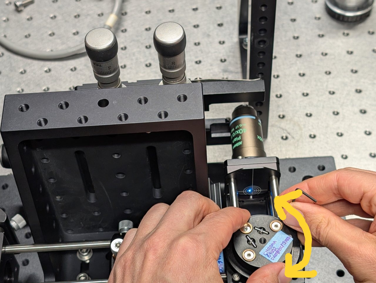
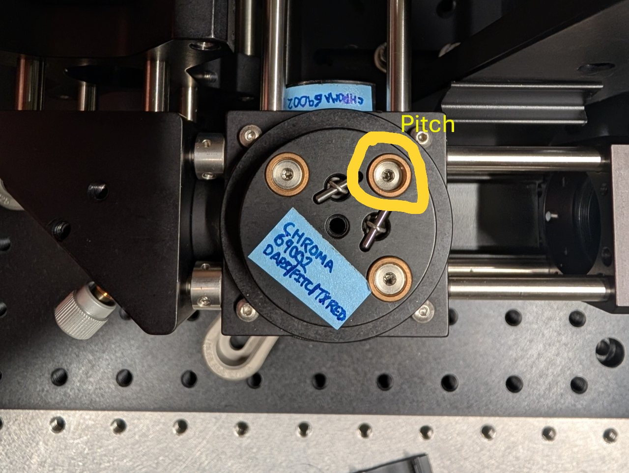
24
Remove the cage plate covers before the objective.
Loosen the screws on the dichroic cube plate. Rotate the entire base plate and adjust the dichroic’s pitch until the beam is roughly centered with respect to the cage rods. Use the alignment plates to determine the beam’s centration.
It is likely that you will not be able to perfectly center the beam with respect to the cage rods because the cube plate does not have the degrees of freedom necessary for full alignment.
Tighten the screws once you come as close to centration with the cage rods as you can.
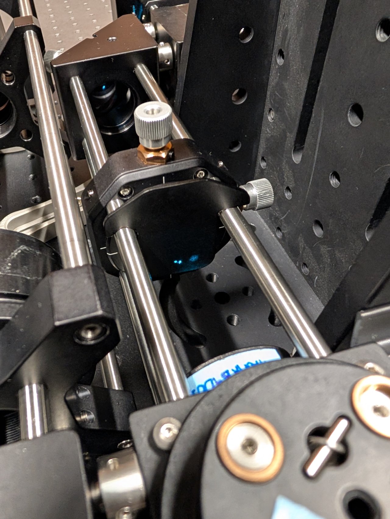
25
Look at the back side of an alignment plate inserted into the 6“ cage rods. Look for back reflections from the objective and excitation filter.
One reflection will come from the excitation filter. It will remain stationary as the dichroic is rotated or the objective is moved.
The other reflections should move with the dichroic or objective. These are from the back reflections from the internal surfaces of the objective.
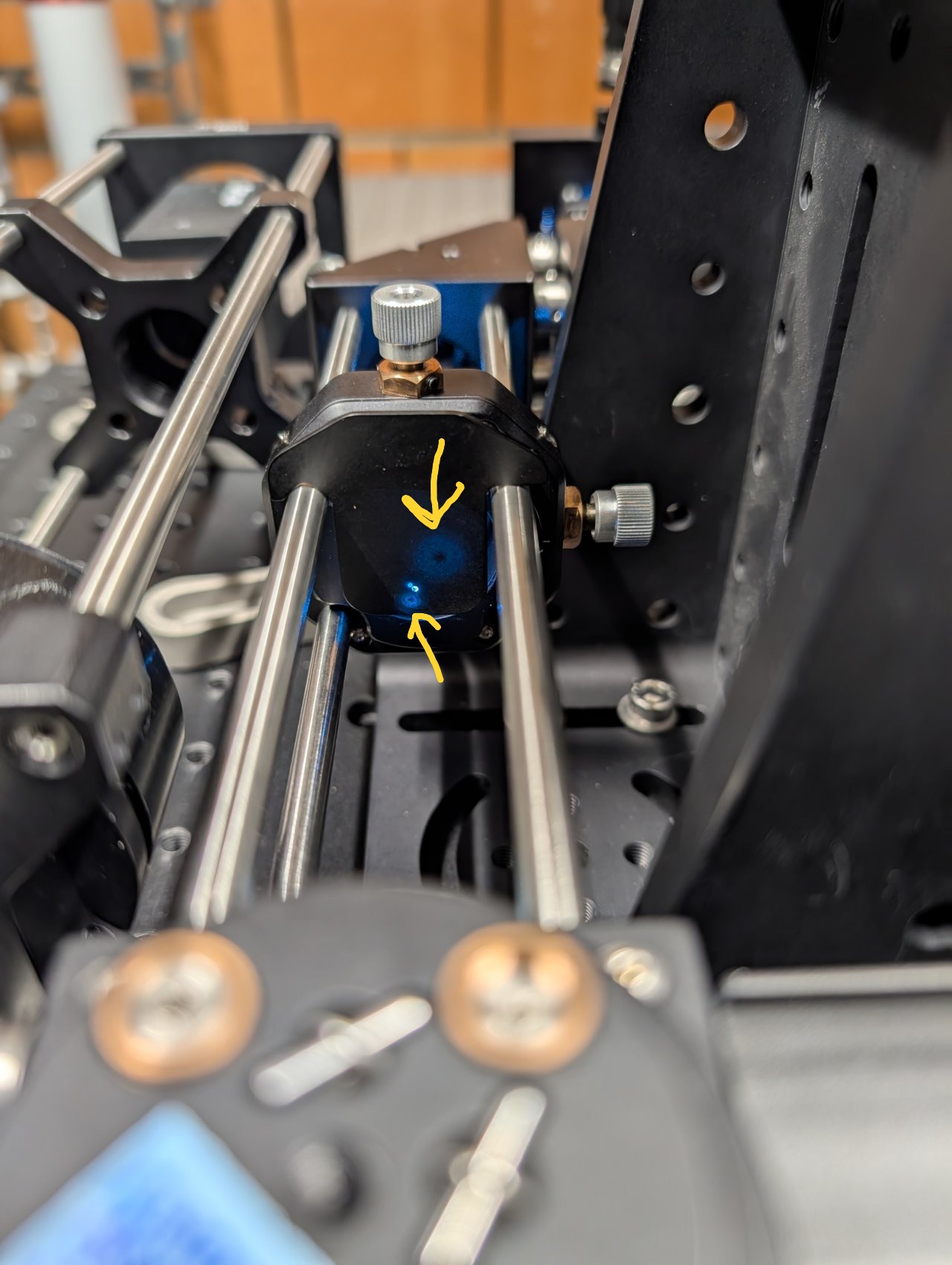
26
To center the back reflections on the alignment plate, you must
- rotate the dichroic, and
- translate the objective using the slip plate.
The objective is well-aligned to the laser beam when the back reflections are centered on the incoming beam.
27
Thread the f = +150 mm achromatic lens into the XY translating lens mount. Ensure that the direction marked \( \infty \) is pointed towards the fiber.
28
Open the iris in front of the fiber output coupler.
29
Put an index card in front of the objective at a distance of about 1 meter or longer.
Slide the f = +150 mm lens along the cage rods until the beam size is minimized.
30
The beam will appear astigmatic due to reflection from the 1 mm thick dichroic. Try to find the lens position. where the beam size is smallest in each direction.
31
Tighten the set screws to lock the lens in place.
32
Stick an alignment plate into the cage system just after the second right-angle turning mirror and observe the back reflections from the f = +150 mm lens.
33
Adjust the lens’s position until the back reflections are as centered as possible on the incoming beam.
34
Reinstall the cage system cover plates before the objective.
Discussion
Astigmatism in the Reflected Beam and Dichroic Thickness
The laser beam becomes astigmatic after it reflects off of the dichroic. This means that the beam’s focal plane in the sample space for one transverse direction is different from its perpendicular direction.
This is a common problem for applicatons requiring laser beam shaping. The solution is to buy thicker dichroics, such as 2 mm or even 3 mm dichroics.
Of course, this comes with tradeoffs. For one, thicker dichroics are more expensive. Additionally, many dichroic mounts are not designed to hold dichroics thicker than 1 mm.
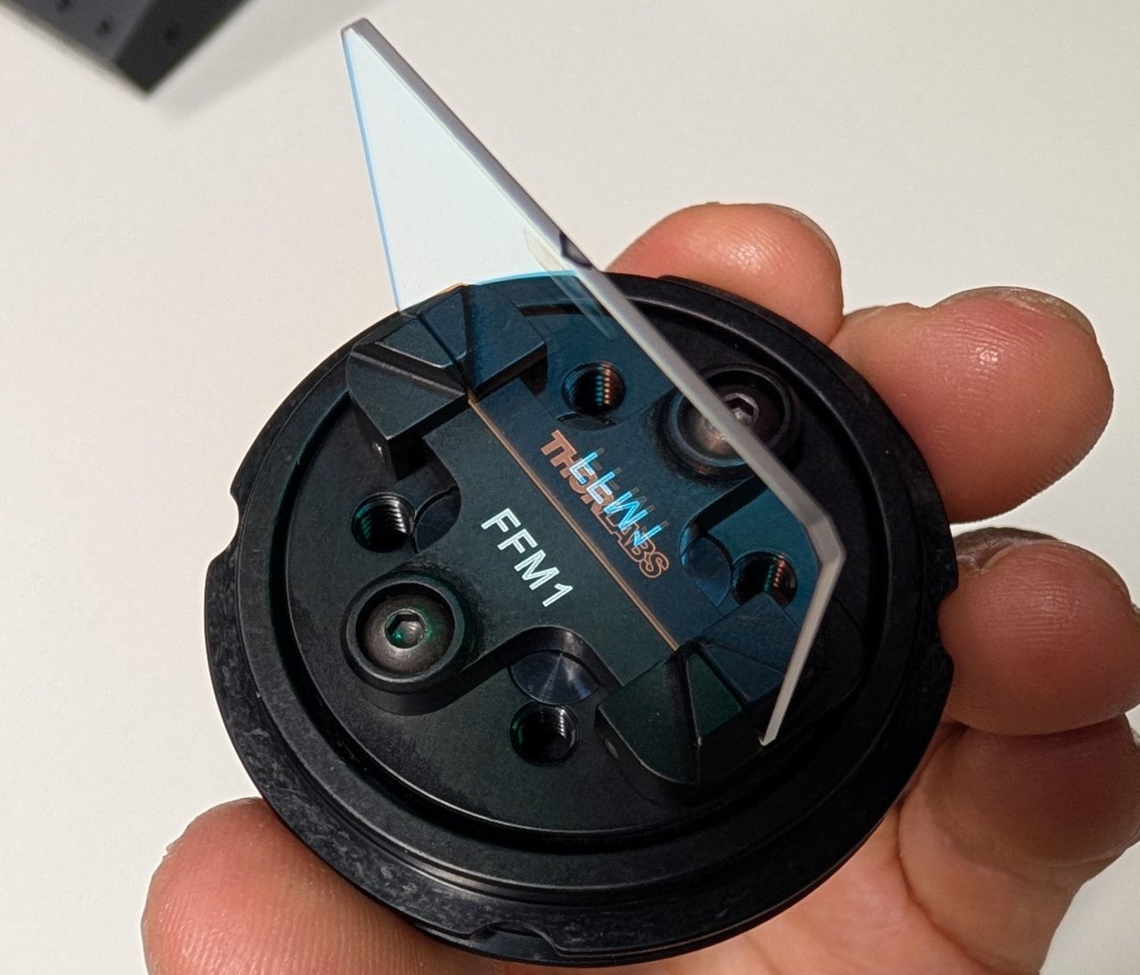
The Thorlabs FFM1 filter holder, mounted inside a cage cube, can hold dichroics up to 3 mm thick and is compatible with kinematic base plates which facilitate alignment.
Further Reading
- Jost AP, Waters JC. Designing a rigorous microscopy experiment: Validating methods and avoiding bias. J Cell Biol. 2019 May 6;218(5):1452-1466. doi: 10.1083/jcb.201812109. Epub 2019 Mar 20. PMID: 30894402; PMCID: PMC6504886. https://doi.org/10.1083/jcb.201812109